echo "This is my course repository for StatProg 2" > README.mdPractical #1
Advanced Statistical Programming using R - Introduction
Quiz
Before starting, work through this QUIZ to check your understanding of the concepts covered in the lecture, as well as preliminary knowledge about R.
General Remarks
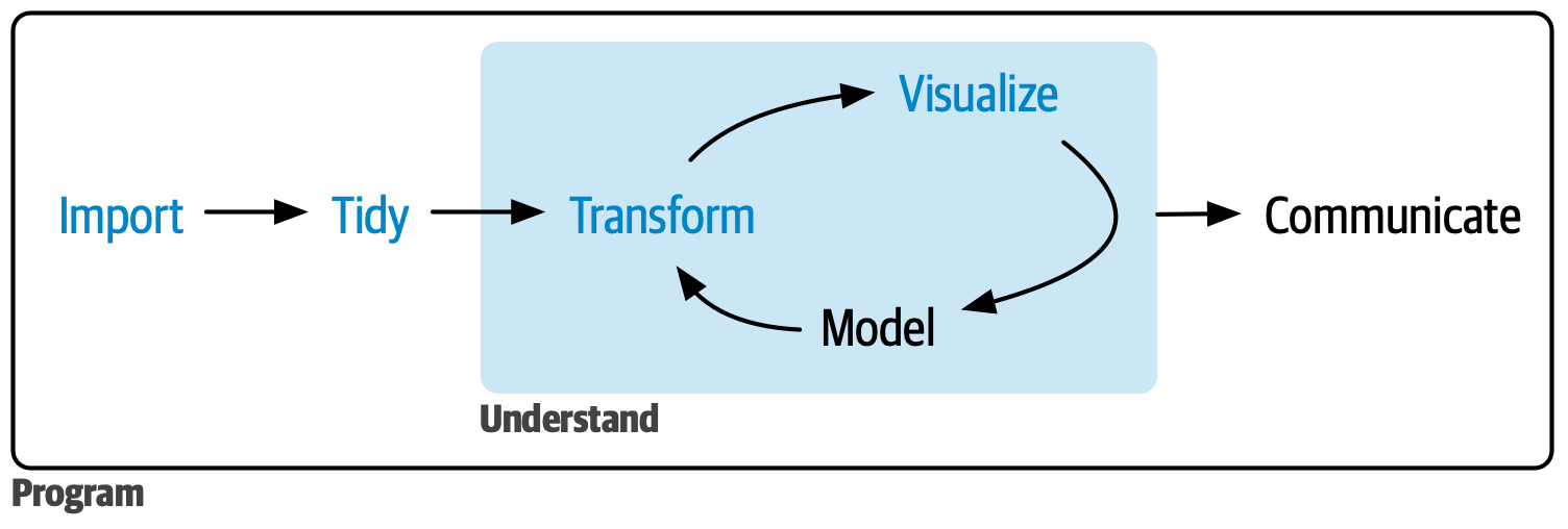
In the first practical session, we will set up all the tools that will be used in this course and practice some basic skills and recap some of the skills from StatProg 1. The learning objectives for this session are:
- Set up all the tools that will be used in this course:
- R, Rstudio, tidyverse installation
- git, GitHub
- Quarto (via R, and command line)
- Command line
- Basic usage of these tools, and how they fit into a data science workflow
- Rendering quarto documents
- Basic command line operations
- Work with Git repositories
- Work with (relative) paths
- Recap of skills from StatProg 1
- Data wrangling (
dplyr) - Data visualisation (
ggplot2)
- Data wrangling (
Exercise 0: Set up your tools
If you successfully finished the “Introduction to Statistical Software for the Statistics Minor” class, you should already have all the tools installed. If not, please follow the instructions below to set up your tools for this course.
- Install R and Rstudio
- Install the tidyverse packages in R:
install.packages("tidyverse")Exercise 1: Command line basics
- Open a command line. You can either do this via Rstudio (Terminal tab) or via your operating system’s terminal application (e.g. Terminal on Mac, Command Prompt or PowerShell on Windows).
If you are new to the command line, here are some basic commands to get you started:
| Description | Windows | Mac/Linux | Example |
|---|---|---|---|
| Change directory | cd <target-directory>1 |
cd <target-directory> |
cd ~/Downloads opens the Downloads folder |
| Display current directory | cd2 |
pwd3 |
pwd displays your current location in the file system |
| List files in directory | dir <target-directory>4 |
ls <target-directory>5 |
ls ~/Downloads lists files in the current directory |
| Create a new directory | mkdir <directory-name>6 |
mkdir <directory-name> |
mkdir my-new-folder creates a new folder called “my-new-folder” in the current directory |
| Remove a directory | rmdir <directory-name>7 |
rmdir <directory-name> |
rmdir my-new-folder removes the folder “my-new-folder” (only if it is empty) |
| Create a new file | type nul > <file-name> |
touch <file-name> |
touch my-file.txt creates a new file called “my-file.txt” in the current directory |
| Display file contents | type <file-name> |
cat <file-name> |
cat my-file.txt displays the contents of the file “my-file.txt” |
| Remove a file | del <file-name>8 |
rm <file-name>9 |
rm my-file.txt removes the file “my-file.txt” |
TipGetting help with CLI commands
On Mac/Linux, man <command> opens the manual page for a command (e.g. man ls). Press q to exit. Most commands also accept a --help flag (e.g. ls --help) for a shorter summary. On Windows, use <command> /? (e.g. dir /?).
Using the command line, navigate to your home directory, create a new folder (directory) for this course and navigate into it.
Using the command line, create a new file called
hello-world.qmdin that folderDisplay the contents of that file in the command line (it should be empty). Add some content to the file (e.g. “Hello, world!”) using RStudio. Display the contents of the file again in the command line to confirm that your changes were saved.
Render the quarto file using the
quarto rendercommand. The command creates an HTML file, which you can display in your browser.You can also render the document using the “Render” button in Rstudio.
Exercise 2: Relative paths
For a deep dive into relative paths and project handling in R, see R4DS Chapter 6 and Q4S Chapter 4.
- Save this image in your course folder and load it in your quarto document using a relative path
- In Markdown images are included like this:
- In R you can include images using
knitr::include_graphics()like this:
knitr::include_graphics("./<image-name>.png")Move the image to a new folder (e.g. create a new folder called “images” and move the image there) and update the path in your quarto document accordingly.10
Move the image outside of your course folder (e.g. to your desktop) and try to load it again using a relative path.11
(Optional) Install the
herepackage (see Q4S Chapter 4.7) and use it to load the image in your quarto document. Theherepackage provides a simple way to construct file paths relative to the root of your project, which can make your code more robust12 and easier to read.
Exercise 3: git repositories
Now, we will set up a git repository for this course and practice some basic git commands. There is a very handy cheat sheet for git commands available here. Take a look at the first three sections of the cheat sheet (Getting Started, Preparing to Commit, and Making Commits).
Initialize a new git repository in your course folder using the command line
git init.Create a new file called
README.mdin your course folder and add some content to it (e.g. “This is my course repository for StatProg 2”). Save the file.13
NoteSolution
You can create the file and add content using RStudio, or you can do it directly in the command line using the echo command:
Use the
git statuscommand to see the status of your repository. You should see that theREADME.mdfile is untracked (i.e. it is not yet being tracked by git).Use the
git addcommand to stage theREADME.mdfile for commit. Then use thegit statuscommand again to see that the file is now staged.
NoteSolution
git add README.md
git status- Use the
git commitcommand to commit the staged file. You will be prompted to enter a commit message.
NoteSolution
You can also provide the commit message directly in the command line using the -m flag:
git commit -m "Add README file"Use the
git logcommand to see the commit history of your repository. You should see your commit with the message you entered.(Optional) Create a new repository on GitHub and push your local repository to GitHub. This will allow you to access your code from anywhere and collaborate with others.
Exercise 4: Descriptive statistics and visualisation
- Load the
palmerpenguinsdataset from thepalmerpenguinspackage and take a look at the data.
NoteSolution
# install.packages("palmerpenguins")
library(palmerpenguins)
head(penguins)
# A tibble: 6 × 8
species island bill_length_mm bill_depth_mm flipper_length_mm body_mass_g
<fct> <fct> <dbl> <dbl> <int> <int>
1 Adelie Torgersen 39.1 18.7 181 3750
2 Adelie Torgersen 39.5 17.4 186 3800
3 Adelie Torgersen 40.3 18 195 3250
4 Adelie Torgersen NA NA NA NA
5 Adelie Torgersen 36.7 19.3 193 3450
6 Adelie Torgersen 39.3 20.6 190 3650
# ℹ 2 more variables: sex <fct>, year <int>- Filter the dataset to include only the
Adeliespecies and create a scatter plot of bill length vs. bill depth usingggplot2. The result should look like this:

NoteSolution
library(tidyverse)
penguins %>%
  filter(species == "Adelie") %>%
  ggplot(aes(x = bill_length_mm, y = bill_depth_mm)) +
  geom_point() +
  labs(title = "Bill Length vs. Bill Depth for Adelie Penguins",
       x = "Bill Length (mm)",
       y = "Bill Depth (mm)")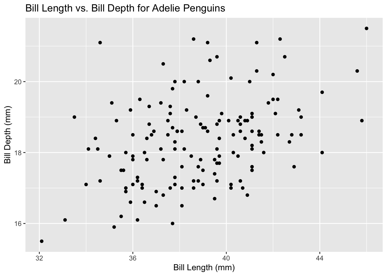
- Calculate some descriptive statistics for the variable
bill_length_mm(e.g. mean, median, standard deviation) usingdplyrfunctions likesummarise(). You can group the data by species or island to see how the statistics differ between groups.
NoteSolution
penguins %>%
  group_by(species) %>%
  summarise(mean_bill_length = mean(bill_length_mm, na.rm = TRUE),
            median_bill_length = median(bill_length_mm, na.rm = TRUE),
            sd_bill_length = sd(bill_length_mm, na.rm = TRUE))
# A tibble: 3 × 4
species mean_bill_length median_bill_length sd_bill_length
<fct> <dbl> <dbl> <dbl>
1 Adelie 38.8 38.8 2.66
2 Chinstrap 48.8 49.6 3.34
3 Gentoo 47.5 47.3 3.08- Create a boxplot of for each numeric variable (
bill_length_mm,bill_depth_mm,flipper_length_mm,body_mass_g) by species to visualize the distributions for each species. How is each species characterised by these features?14
NoteSolution
penguins %>%
  pivot_longer(cols = c(bill_length_mm, bill_depth_mm, flipper_length_mm, body_mass_g),
               names_to = "feature",
               values_to = "value") %>%
  ggplot(aes(x = species, y = value)) +
  geom_boxplot() +
  facet_wrap(~ feature, scales = "free_y") +
  labs(title = "Boxplots of Penguin Features by Species",
       x = "Species",
       y = "Value")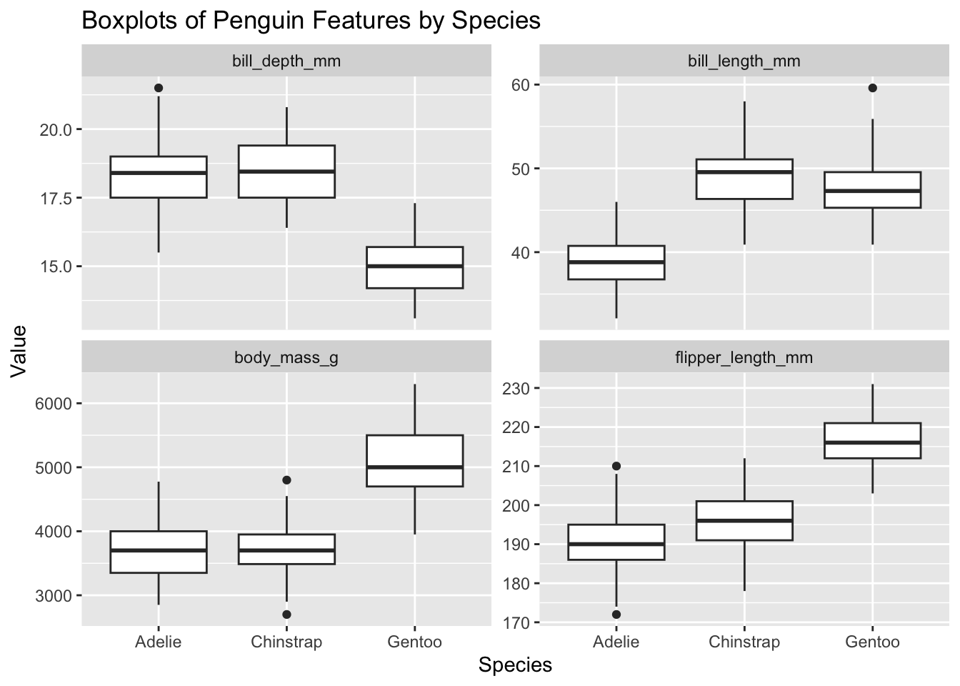
References
- R4DS Chapter 1-10 - R for Data Science (2e) by Hadley Wickham, Mine Çetinkaya-Rundel, and Garrett Grolemund
- Q4S Chapter 4 - Quarto for Scientists by Nicholas J. Tierney
Footnotes
Change Directory↩︎
In Windows, the Change Directory command without arguments prints the current directory↩︎
Print Working Directory↩︎
Directory↩︎
List↩︎
Make Directory↩︎
Remove Directory↩︎
Delete↩︎
Remove↩︎
This simulates a common workflow where you have different folders for different types of files (e.g. data, images, scripts, etc.) and need to update paths when you move files around.↩︎
In some cases, this will not work, because the image is now outside of your project folder and cannot be accessed using a relative path. This highlights the importance of keeping all your project files within a single folder structure and using relative paths to access them.↩︎
Robust means your code will run on any machine regardless of operating system and environment↩︎
The README file is a common file in git repositories that provides an overview of the project and its contents.↩︎
You can either create multiple plots for this task or try to visualise everything in one plot using faceting in ggplot2.↩︎