f1 <- function(string, prefix) {
  str_sub(string, 1, str_length(prefix)) == prefix
}

f3 <- function(x, y) {
  rep(y, length.out = length(x))
}Practical #2
Advanced Statistical Programming using R - Introduction
ImportantAnnouncement
THE PRACTICAL NEXT WEEK WILL BE ON THURSDAY, APRIL 30th, RIGHT AFTER THE LECTURE!!
Since May 1st is a public holiday, we needed to reschedule.
Quiz
Before starting, work through this QUIZ to check your understanding of the concepts covered in the lecture, as well as preliminary knowledge about R.
General Remarks
In this practical, we will take a look at how to write functions in R, and why they are useful for data science tasks. We will cover the following topics:
- Naming conventions for functions and their arguments
- Why is it important to choose meaningful names for functions and their arguments?
- What are some common naming conventions in R (e.g. snake_case, camelCase, etc.) and when should you use them?
- Refactoring code into functions to make it more modular and reusable
- How can you identify which parts of your code can be turned into functions?
- What are the benefits of refactoring code into functions (e.g. improved readability, easier maintenance, reusability)?
- Error handling in functions
- How can you use mechanisms such as
stop()to handle errors in your functions? - What are some best practices for error handling in R (e.g. providing informative error messages, using assertions to check input validity)?
- Recursion and iteration
- What is the difference between recursion and iteration, and when should you use each approach?
- How can you implement recursive functions in R, and what are some common pitfalls to avoid (e.g. stack overflow errors)?
Exercise 1: Naming Functions
A good function name is a verb or short phrase that tells you what the function does without having to read its body. Badly named functions (f1, do_stuff, helper2) force every reader — including future-you — to re-derive intent from the code each time.
The exercises below are adapted from R4DS, Chapter 26.
- Read the source code for each of the following two functions, puzzle out what they do, and then brainstorm better names.
NoteSolution
f1checks whetherstringstarts withprefix. A better name isstarts_with_prefix()or justhas_prefix(). (This is essentially whatstringr::str_starts()does.)f3recyclesyso that its length matchesx. A better name isrecycle_to_length()ormatch_length().
In both cases the new name is a verb phrase: you should be able to read has_prefix(string, prefix) as a small English sentence.
- Make a case for why
norm_r(),norm_d()etc. would be better thanrnorm(),dnorm()1. Make a case for the opposite. How could you make the names even clearer?
NoteExample Arguments
For norm_r() / norm_d(): groups all normal-distribution functions under a common prefix, which is great for autocomplete — typing norm_ in RStudio would show you every related function.
For rnorm() / dnorm(): follows a long-standing R convention (r = random, d = density, p = cumulative, q = quantile) that is shared across all distributions (rbinom, dbinom, rbeta, …). Breaking this convention in one place adds friction everywhere else.
Even clearer might be something like normal_sample(), normal_density(), normal_cdf(), normal_quantile() — fully spelt-out verbs, at the cost of more typing.
Exercise 2: Using Functions to Package Code
Last week you wrote a bit of code to filter and plot the palmerpenguins data. Copy-pasting that code every time you want the same plot for a different species is a recipe for bugs — the moment you change one copy and forget the others, your plots start disagreeing. Turning the code into a function fixes this: there is one place that defines the behaviour, and you invoke it with different arguments.
- Take a look at the following code. Wrap this code in a function with a fitting name and appropriate arguments.
library(palmerpenguins)
library(tidyverse)

penguins %>%
  filter(species == "Adelie") %>%
  ggplot(aes(x = bill_length_mm, y = bill_depth_mm)) +
  geom_point() +
  labs(title = "Bill Length vs. Bill Depth for Adelie Penguins",
       x = "Bill Length (mm)",
       y = "Bill Depth (mm)")
TipHint
What pieces of this code would you want to vary between calls? The species is an obvious candidate. What about the two axis variables? And the title?
- Add a docstring to your function that explains what the function does, its arguments, and its return value.
TipHint
In R, docstrings are written as comments starting with #' directly above the function definition, using roxygen2 tags like @param, @return, @examples. See the solution to Exercise 7 below for a fuller example.
NoteSolution
library(palmerpenguins)
library(tidyverse)

#' Plot two numeric penguin features against each other, filtered by species.
#'
#' @param species The penguin species to keep (e.g. "Adelie", "Gentoo", "Chinstrap").
#' @param x_var   Name of the column to plot on the x-axis (default: "bill_length_mm").
#' @param y_var   Name of the column to plot on the y-axis (default: "bill_depth_mm").
#' @return A ggplot object.
scatter_penguins <- function(penguin_species,
                               x_var = "bill_length_mm",
                               y_var = "bill_depth_mm") {
  penguins %>%
    filter(species == penguin_species) %>%
    ggplot(aes(x = .data[[x_var]], y = .data[[y_var]])) +
      geom_point() +
      labs(title = paste(x_var, "vs.", y_var, "for", penguin_species, "penguins"),
          x = x_var,
          y = y_var)
}

scatter_penguins("Adelie")
scatter_penguins("Gentoo", x_var = "flipper_length_mm", y_var = "body_mass_g")
Note the use of .data[[ ]] and .env$ — these are tidy evaluation helpers that let you pass column names as plain strings. We will come back to this in a later lecture.
Test your function by calling it with different arguments and checking the output. Make sure to test edge cases:
- What happens if you pass in a species name that doesn’t exist (e.g.
"Penguin")? - What happens if you pass a column name that isn’t in the data (e.g.
x_var = "fluffiness")? - What happens if you pass a non-numeric column (e.g.
x_var = "island")?
Write down what you expect to happen for each case before running it — are the actual errors informative? We’ll fix the bad ones in Exercise 3.
- What happens if you pass in a species name that doesn’t exist (e.g.
Split your function into smaller helper functions. One function should only perform one task.
Then rewrite
scatter_penguins()to just call these two helpers in sequence. The top-level function becomes shorter and easier to read, and each helper is independently testable.
NoteExample Solution
#' Return a scatter plot of two variables
#'
#' @param data    Dataset
#' @param x_var   Name of the column to plot on the x-axis.
#' @param y_var   Name of the column to plot on the y-axis.
#' @return A ggplot object.
scatter_plot <- function(data, x_var, y_var) {
  ggplot(data, aes(x = .data[[x_var]], y = .data[[y_var]])) +
    geom_point() +
    labs(title = paste(x_var, "vs.", y_var),
        x = x_var,
        y = y_var)
}

#' Plot two numeric penguin features against each other, filtered by species.
#'
#' @param species The penguin species to keep (e.g. "Adelie", "Gentoo", "Chinstrap").
#' @param x_var   Name of the column to plot on the x-axis (default: "bill_length_mm").
#' @param y_var   Name of the column to plot on the y-axis (default: "bill_depth_mm").
#' @return A ggplot object.
scatter_penguins_with_helper <- function(penguin_species,
                               x_var = "bill_length_mm",
                               y_var = "bill_depth_mm") {
  penguins %>%
    filter(species == penguin_species) %>%
    scatter_plot(x_var, y_var)
}

scatter_penguins_with_helper("Adelie")
scatter_penguins_with_helper("Gentoo", x_var = "flipper_length_mm", y_var = "body_mass_g")
Exercise 3: Error Handling
In Exercise 2, you probably noticed that passing a non-existent species name returns an empty plot with no explanation, and passing a bad column name gives a cryptic object not found error. A well-written function should fail fast with an informative message rather than produce silently broken output.
R has a few tools for this:
stop("message")throws an error with a custom message.stopifnot(condition1, condition2, ...)throws an error if any condition isFALSE. It’s a compact way to write several assertions at the top of a function.- (Extension)
cli::cli_abort()produces prettier, multi-line error messages with argument highlighting — it’s what the tidyverse uses internally.
Tasks
- Add input validation to your function from Exercise 2 so that it fails with a useful message when:
speciesis not one of the three valid species ("Adelie","Chinstrap","Gentoo").x_varory_varis not a column of thepenguinsdata frame.x_varory_varrefers to a non-numeric column.
NoteSolution
scatter_penguins <- function(species,
                               x_var = "bill_length_mm",
                               y_var = "bill_depth_mm") {
  valid_species <- c("Adelie", "Chinstrap", "Gentoo")
  if (!species %in% valid_species) {
    stop("`species` must be one of: ", paste(valid_species, collapse = ", "),
         ". You supplied: \"", species, "\".")
  }

  stopifnot(
    "`x_var` must be a column of `penguins`" = x_var %in% names(penguins),
    "`y_var` must be a column of `penguins`" = y_var %in% names(penguins),
    "`x_var` must be numeric"                = is.numeric(penguins[[x_var]]),
    "`y_var` must be numeric"                = is.numeric(penguins[[y_var]])
  )

  penguins %>%
    filter(species == .env$species) %>%
    ggplot(aes(x = .data[[x_var]], y = .data[[y_var]])) +
    geom_point() +
    labs(title = paste(x_var, "vs.", y_var, "for", species, "penguins"),
         x = x_var, y = y_var)
}

scatter_penguins("Emperor", "x", "y")
scatter_penguins("Adelie", "x", "y")
scatter_penguins("Adelie", "bill_length_mm", "species")
Notice how named elements of stopifnot() double as error messages — this is often enough for small functions.
- Compare the error messages you get now vs. before. Which version would be easier to debug at 11pm the night before an assignment deadline?
TipExtension: better errors with
cli
The cli package (covered in the lecture) lets you write multi-line error messages with argument highlighting:
library(cli)
if (!species %in% valid_species) {
  cli_abort(c(
    "{.arg species} must be one of {.val {valid_species}}.",
    "x" = "You supplied {.val {species}}."
  ))
}
This is the style used throughout the tidyverse.
Exercise 4: Recursion and Iteration
In this section we’ll take a look at how to compute 2 raised to the power of 10 (\(2^{10}\)). There are two common approaches to solve this problem:
Approach 1: Repeat 10 Times
\(2^{10}\) can be computed by multiplying 2 by itself 10 times: \(\Pi_{i=1}^{10} 2 = 2 * 2 * 2 * 2 * 2 * 2 * 2 * 2 * 2 * 2 = 1024\). This is an example of iteration, where we repeat an operation a certain number of times.
TipIteration
Iteration is a programming technique where a block of code is repeated a certain number of times or until a certain condition is met. An iterative function typically uses loops (e.g. for, while).
- The same function \(f(a, b) = a^b\) can be implemented iteratively as follows:
- we initialize a variable
resultto 1 - Then, in a loop that runs
btimes, - we multiply result by
a.
- we initialize a variable
# Example of an iterative function to compute a to the power of b
power_iterative <- function(a, b) {
  # We initialize a variable `result` to 1, which will hold the final result of a^b.
  result <- 1
  # Then, we use a for loop that runs `b` times.
  # 1:b creates a sequence of numbers from 1 to b, and the loop iterates over this sequence.
  for (i in 1:b) {
    # In each iteration, we update `result` by multiplying it with `a`.
    # After the loop finishes, `result` will contain the value of a^b.
    result <- result * a
  }
  # Finally, we return the computed result.
  return(result)
}
power_iterative(2, 3) # This will compute 2^3 = 8
Iteration can be more efficient and avoid stack overflow errors, but it can also be less elegant and harder to read.
Approach 2: Well, I know \(2^9\) …
\(2^{10}\) can also be computed as \(2 * 2^9 = 2 * (2 * 2^8) = 2 * (2 * (2 * 2^7))\), and so on, until we reach the base case of \(2^0 = 1\). Formally, we have \(2^{n} = 2 * 2^{n-1}\) if \(n > 0\), and \(2^{0} = 1\). This is an example of recursion, where a function calls itself to solve a problem.
TipRecursion
Recursion is a programming technique where a function calls itself in order to solve a problem. A recursive function typically consists of a recursive case (also called the recursion step) that breaks the problem into smaller subproblems and a base case that stops the recursion.
- Take the function \(f(a, b) = a^b\)
- This function can be implemented recursively as follows:
- Base case \(f(a, 0) = 1\)
- Recursive case \(f(a, b) = a * f(a, b-1)\)
# Example of a recursive function to compute a to the power of b
power_recursive <- function(a, b) {
  if (b == 0) {
    # This is the so called base case, which is necessary to prevent infinite recursion
    # It defines, when the function should stop calling itself and return a value.
    # In this case, any number to the power of 0 is 1, so we return 1.
    return(1)
  } else {
    # This is the recursion step, where the function calls itself with modified arguments.
    # In this case, we multiply `a` by the result of calling `power_recursive` with `b`
    # decremented by 1, which effectively reduces the problem size with each recursive call.
    return(a * power_recursive(a, b - 1))
  }
}

power_recursive(2, 3) # This will compute 2^3 = 8
Recursion can be more elegant and easier to read, but it can also be less efficient and lead to stack overflow errors if the recursion depth is too large.
Task: The Fibonacci Sequence
Do you remember the Fibonacci sequence from your math classes? The Fibonacci sequence is defined as follows:
- \(F(0) = 0\), \(F(1) = 1\), and \(F(n) = F(n-1) + F(n-2)\) for \(n > 1\), so:
- \(F(2) = F(1) + F(0) = 1 + 0 = 1\)
- \(F(3) = F(2) + F(1) = 1 + 1 = 2\)
- \(F(4) = F(3) + F(2) = 2 + 1 = 3\)
- \(F(5) = F(4) + F(3) = 3 + 2 = 5\)
- …
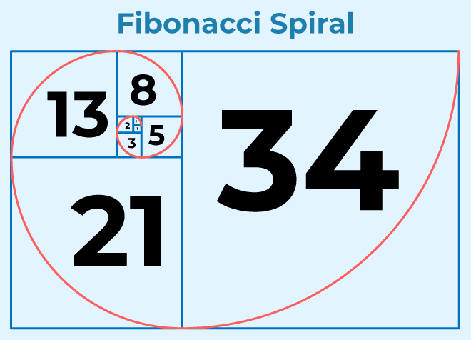
The Fibonacci sequence is a classic example of a problem that can be solved using both iteration and recursion, and it illustrates the trade-offs between these two approaches.
- Write a function in R to compute the nth Fibonacci number iteratively.
NoteSolution
fib_iterative <- function(n) {
  if (n == 0) {
    return(0)
  } else if (n == 1) {
    return(1)
  } else {
    a <- 0
    b <- 1
    for (i in 2:n) {
      temp <- a + b
      a <- b
      b <- temp
    }
    return(b)
  }
}- Write a function in R to compute the nth Fibonacci number recursively.
NoteSolution
fib_recursive <- function(n) {
  if (n == 0) {
    return(0)
  } else if (n == 1) {
    return(1)
  } else {
    return(fib_recursive(n - 1) + fib_recursive(n - 2))
  }
}- Compare the performance of the iterative and recursive implementations by computing the 30th Fibonacci number. What is the difference? Why does this difference occur?
NoteSolution
system.time(fib_iterative(35)) # This will compute the 35th Fibonacci number, which is 9227465
system.time(fib_recursive(35)) # This will compute the 35th Fibonacci number, which is 9227465
The iterative implementation is much faster than the recursive implementation for computing the 35th Fibonacci number. This difference occurs because the recursive implementation has a lot of redundant calculations. For example, to compute F(35), the recursive function will compute F(34) and F(33), and to compute F(34), it will compute F(33) and F(32), and so on. This leads to an exponential growth in the number of function calls, which makes the recursive implementation very inefficient for larger values of n.
The iterative implementation, on the other hand, computes each Fibonacci number from 2 up to n exactly once, resulting in a linear time complexity. Therefore, the iterative implementation is much more efficient for larger values of n.
Note: Recursion is not always inefficient. In some cases, it can lead to elegant and easy-to-read code. However, for problems like the Fibonacci sequence, where there are many overlapping subproblems, an iterative approach or memoization (caching previously computed results) can significantly improve performance. This illustrates the importance of choosing the right approach based on the problem at hand.
Exercise 5: Refactoring
A guiding principle: DRY — Don’t Repeat Yourself. If the same block of code appears in more than one place, there’s one behaviour with multiple copies. Change one, forget the others, and they drift out of sync.
Task 1: Spot the repetition
Consider the following function that produces a small summary for a single species:
summarise_species <- function(species_name) {
  adelie_mean_bill <- mean(penguins$bill_length_mm[penguins$species == "Adelie"], na.rm = TRUE)
  gentoo_mean_bill <- mean(penguins$bill_length_mm[penguins$species == "Gentoo"], na.rm = TRUE)
  chinstrap_mean_bill <- mean(penguins$bill_length_mm[penguins$species == "Chinstrap"], na.rm = TRUE)

  adelie_mean_mass <- mean(penguins$body_mass_g[penguins$species == "Adelie"], na.rm = TRUE)
  gentoo_mean_mass <- mean(penguins$body_mass_g[penguins$species == "Gentoo"], na.rm = TRUE)
  chinstrap_mean_mass <- mean(penguins$body_mass_g[penguins$species == "Chinstrap"], na.rm = TRUE)

  if (species_name == "Adelie") {
    cat("Adelie — mean bill:", adelie_mean_bill, "mean mass:", adelie_mean_mass, "\n")
  } else if (species_name == "Gentoo") {
    cat("Gentoo — mean bill:", gentoo_mean_bill, "mean mass:", gentoo_mean_mass, "\n")
  } else if (species_name == "Chinstrap") {
    cat("Chinstrap — mean bill:", chinstrap_mean_bill, "mean mass:", chinstrap_mean_mass, "\n")
  }
}- Identify every piece of repetition in this function. How many distinct ideas are actually being expressed?
- Rewrite the function so that:
- the per-species means are not hard-coded,
- there’s no long
if/elsechain onspecies_name, - the code would still work if a fourth species showed up in the data.
NoteExample Solution
summarise_species <- function(species_name, data = penguins) {
  row <- data %>%
    filter(species == species_name) %>%
    summarise(mean_bill = mean(bill_length_mm, na.rm = TRUE),
              mean_mass = mean(body_mass_g,    na.rm = TRUE))

  cat(species_name,
      "— mean bill:", row$mean_bill,
      "mean mass:",   row$mean_mass, "\n")
}

summarise_species("Adelie")
summarise_species("Gentoo")
The new version has no per-species repetition and automatically handles any species present in the data.
Task 2: Refactor a long function into helpers
Take the following monolithic function. It loads a dataset, cleans it, summarises it, and plots it — all in one place.
penguin_report <- function(species_name) {
  # load
  library(palmerpenguins)
  library(tidyverse)
  data <- penguins

  # clean
  data <- data[!is.na(data$bill_length_mm) & !is.na(data$body_mass_g), ]

  # filter
  data <- data[data$species == species_name, ]

  # summarise
  cat("n =", nrow(data), "\n")
  cat("mean bill length:", mean(data$bill_length_mm), "\n")
  cat("mean body mass:",   mean(data$body_mass_g),    "\n")

  # plot
  ggplot(data, aes(x = bill_length_mm, y = body_mass_g)) +
    geom_point() +
    labs(title = paste("Bill length vs. body mass —", species_name))
}

penguin_report("Gentoo")
Refactor it into at least three helper functions. Each helper should do one thing, and the top-level penguin_report() should read like a recipe: load, then clean, then summarise, then plot.
TipHint
Good candidate helpers:
load_penguins()— returns the raw dataset.drop_missing(data, cols)— drops rows withNAin the given columns.print_summary(data)— printsn, mean bill length, mean body mass.scatter_bill_vs_mass(data, title)— returns a ggplot.
Once these exist, penguin_report() becomes three or four lines.
NoteSolution
load_penguins <- function() {
  palmerpenguins::penguins
}

drop_missing <- function(data, cols) {
  data[complete.cases(data[, cols]), ]
}

print_summary <- function(data) {
  cat("n =", nrow(data), "\n")
  cat("mean bill length:", mean(data$bill_length_mm), "\n")
  cat("mean body mass:",   mean(data$body_mass_g),    "\n")
}

scatter_bill_vs_mass <- function(data, title) {
  ggplot(data, aes(x = bill_length_mm, y = body_mass_g)) +
    geom_point() +
    labs(title = title)
}

penguin_report <- function(species_name) {
  data <- load_penguins() %>%
    drop_missing(c("bill_length_mm", "body_mass_g")) %>%
    filter(species == species_name)

  print_summary(data)
  scatter_bill_vs_mass(data, title = paste("Bill length vs. body mass —", species_name))
}

penguin_report("Adelie")
Each helper is now independently testable, and the top-level function reads top-to-bottom as the story of the analysis.
Exercise 6: Reflection Log
- Take some time to write this week’s reflection log.
- Add and commit your reflection log to your Git repository (the one we initialized last week).
(Optional) Exercise 7: Freestyle
Write a function that takes the starwars dataset as input and performs some data transformation and visualization tasks. You can choose any dataset and any transformations/visualizations you like. The goal is to practice writing functions that are useful for data science tasks.
Follow these principles when writing your function: - Modularity: Don’t put one large bulk of code in one function. Instead, break it down into smaller helper functions that perform specific tasks. This will make your code easier to read and maintain. - Documentation: Add docstrings to your functions that explain what the function does, its arguments, and its return value. This will make it easier for others (or yourself in the future) to understand how to use the function. - Testing: Test each function with different inputs to ensure it works correctly. Consider edge cases (e.g. empty datasets, missing values) to make sure your function is robust. - Reusability: Design your functions to be reusable in different contexts. Avoid hardcoding specific values or assumptions that limit the function’s applicability. Instead use parameters to allow for flexibility in how the function can be used. E.g. - instead of hardcoding the name of a column to plot, allow the user to specify which column they want to visualize. - instead of hardcoding the type of plot, allow the user to specify which type of plot they want to create (e.g. scatter plot, bar plot, histogram).
CautionHint
Start with writing down the code and then identify which parts of the code can be turned into functions. For example, you might have a block of code that loads the data, another block that performs data transformations, and another block that creates a plot. Each of these blocks can be turned into a separate function. Then, you can write a main function that calls these helper functions in sequence to perform the entire analysis. This way, you can reuse the helper functions in other contexts, and your main function will be easier to read and understand.
NoteExample Solution
library(dplyr)
library(ggplot2)

#' Helper function to load the starwars dataset
#' @return The starwars dataset
load_starwars <- function() starwars # This notation might look odd, but it is a valid way to return the starwars dataset as a function output. The `starwars` dataset is a built-in dataset in R, and by calling it as a function, we are simply returning the dataset when `load_starwars()` is called.

#' Helper function to transform the starwars dataset
#' @param data The input dataset
#' @param x_col The column to use for the x-axis
#' @param y_col The column to use for the y-axis
#' @param color_col The column to use for coloring the points
#' @return A transformed dataset with the specified columns and a new column indicating whether the y value is above average
transform_starwars <- function(data, x_col, y_col, color_col) {
  df <- data.frame(
    x = data[[x_col]],
    y = data[[y_col]],
    color = data[[color_col]],
    y_above_average = data[[y_col]] > mean(data[[y_col]], na.rm = TRUE)
  )
  return(df)
}

#' Example function that takes the starwars dataset and creates a scatter plot of height vs mass, colored by species
#' @param x_col The column to use for the x-axis (default: "height")
#' @param y_col The column to use for the y-axis (default: "mass")
#' @param color_col The column to use for coloring the points (default: "species")
#' @param plot_type The type of plot to create (default: "scatter", options: "scatter", "bar", "histogram")
#' @return A ggplot object representing the specified plot
plot_starwars <- function(x_col = "height", y_col = "mass", color_col = "species", plot_type = "scatter") {
  # This is a helper function that loads the starwars dataset
  data <- load_starwars()

  # Check if the specified columns exist in the dataset
  if (!all(c(x_col, y_col, color_col) %in% colnames(data))) {
    stop("One or more specified columns do not exist in the dataset.")
  }

  # Transform the data as needed for the plot (e.g. create a new column for whether y is above average)
  data_transformed <- transform_starwars(data, x_col, y_col, color_col)

  # Create the plot based on the specified plot type
  if (plot_type == "scatter") {
    p <- ggplot(data_transformed, aes(x = x, y = y, color = color, size = y_above_average)) +
      geom_point() +
      labs(title = paste("Scatter plot of", x_col, "vs", y_col, "colored by", color_col))
  } else if (plot_type == "bar") {
    p <- ggplot(data_transformed, aes_string(x = color, fill = color)) +
      geom_bar() +
      labs(title = paste("Bar plot of", color_col))
  } else if (plot_type == "histogram") {
    p <- ggplot(data_transformed, aes_string(x = x)) +
      geom_histogram() +
      labs(title = paste("Histogram of", x_col))
  } else {
    stop("Invalid plot type specified. Please choose 'scatter', 'bar', or 'histogram'.")
  }
  return(p)
}

# Example usage:
plot_starwars(x_col = "height", y_col = "mass", color_col = "species", plot_type = "scatter")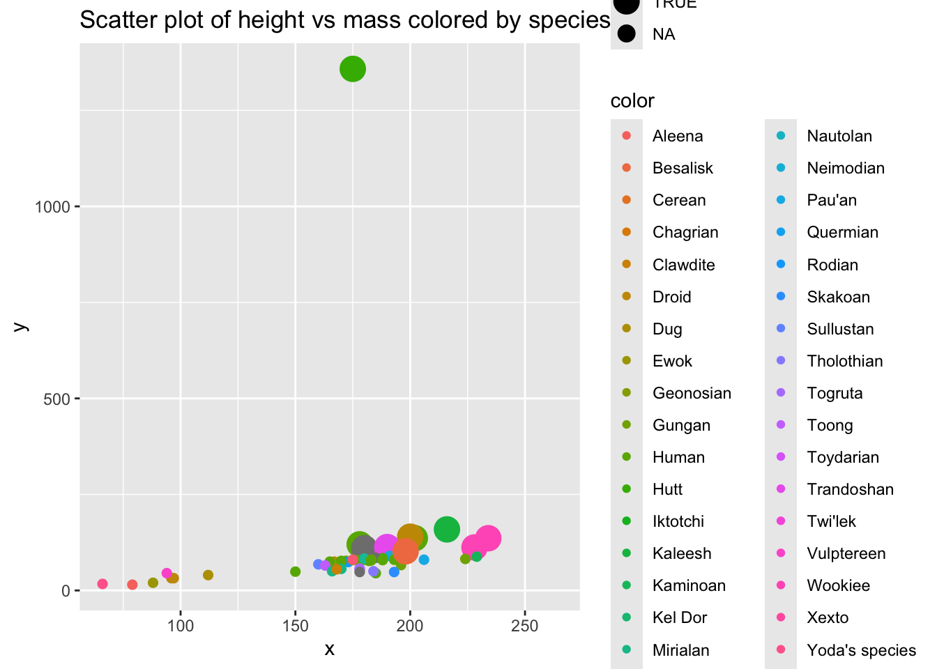
Resources
- R4DS Ch. 25–27: Functions, Iteration
- Advanced R, Ch. 6: Functions (depth reference)
- https://fun2debug.njtierney.com - A blog by Nicholas J. Tierney about writing functions in R, with a focus on making them easy to debug and maintain.
Footnotes
rnorm()generates random numbers from the normal distribution, anddnorm()computes the density (probability density function) of the normal distribution.↩︎