Advanced Statistical Programming using R

Week 2: Scripts, Functions & Refactoring

2026-04-22

Reminders

Register for course on module (see email)
Bookmark course website: https://soda-lmu.github.io/StatProg2-2026-SoSe/
Follow installation & setup requirements: https://soda-lmu.github.io/StatProg2-2026-SoSe/setup.html
Check the updated schedule for changes due to holidays: https://soda-lmu.github.io/StatProg2-2026-SoSe/#schedule

Contact Us

For individual questions: statprog[@]stat.uni-muenchen.de For course related questions: https://moodle.lmu.de/mod/forum/view.php?id=2498223

Last Week

Introduction to the course
Reviewed the data science workflow
Crash course in git & CLI

Reviewing RStudio with the Knife / Kitchen analogy

R = the knife (the tool that actually cuts/does the work)
RStudio = the kitchen (workspace, counters, cupboards)
R Script = the recipe card you write ahead of time
Console = the stove / cooking zone (where you execute the cooking)
Terminal = talks to the kitchen manager (code outside of R, on your whole computer)
R Markdown/Quarto = the cookbook page (with recipe + photos + notes)
File paths = locations of ingredients (R scripts, data, images)
- absolute vs. relative

Command Line

Navigate

pwd          # where am I?
ls           # what's here?
cd <dir>     # move into a folder
cd ..        # move up one level

Create & remove

mkdir <dir>  # new folder
touch <file> # new empty file
rm <file>    # delete a file

Inspect & run

cat <file>          # print file contents
quarto render <file> # render a .qmd

Get help

man <command>   # full manual (Mac/Linux)
<command> --help

Tip

Windows uses cd for pwd, dir for ls, type for cat, and del for rm.

Git for version history

Set up & inspect

git init               # start tracking a folder
git status             # what has changed?
git log                # history of commits

Stage & commit

git add <file>         # stage a file
git add .              # stage all changes
git commit -m "msg"    # save a snapshot

The three areas

working directory  →  staging area  →  repository
   (your files)       (git add)        (git commit)

Think of it as:

Edit files as normal
Stage the changes you want to keep (git add)
Commit a named snapshot (git commit)

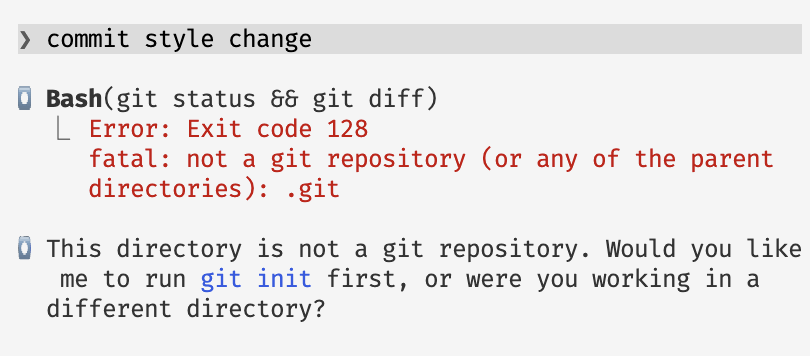
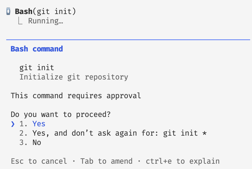
Why command line git?

Safety first (with agentic models)!

This Week

Individual reflection log – git practice!
Reviewing functions in R
Testing functions
Writing (better) functions (for data science tasks)

Individual Reflection Log

See “Reflection Prompts” on the course website

The reflection log lives in the same git repository you set up in last week’s practical
Each week you’ll answer a small set of prompts tracking what you learned around the course
Each answer is committed as a separate commit — practising the version control workflow from day one

Tip

Find this week’s prompts on the course website under Reflection Prompts. Use the provided prompts or write your own and add to individual-reflection-log.qmd. Make sure to commit each week!

Review: Writing Functions

From StatProg 1

What are functions?

A function is a reusable block of code designed to perform a specific task. It takes input (arguments), processes it, and returns output (or performs an action).

Why use functions?

Avoid repeating yourself (DRY)
Easier to test and debug in isolation
Give a name to a chunk of logic

Examples

Function	Input	Action	Output
`sum(a, b)`	two numbers	`a + b`	the sum
`print(x)`	any object	display it	(side effect)
`ggplot(df, aes(...))`	data + aesthetics	build a plot	plot object

Defining a function in R

Step 1: working interactive code

library(palmerpenguins)

max(penguins$bill_length_mm, na.rm = TRUE) -
  min(penguins$bill_length_mm, na.rm = TRUE)
#> [1] 27.5

Step 2: wrap it in a function — add NO new functionality

max_minus_min <- function(x) {
  max(x, na.rm = TRUE) - min(x, na.rm = TRUE)
}

Step 3: check it gives the same answer

max_minus_min(penguins$bill_length_mm)
#> [1] 27.5

Step 4: try it on other columns

max_minus_min(penguins$flipper_length_mm)
max_minus_min(penguins$body_mass_g)

Function syntax in R

Part	Name	What it does
`my_function`	function name	how you call it
`function(...)`	signature	declares the function
`arg1, arg2`	formals / parameters	inputs the function accepts
`arg2 = default`	default value	used when argument is omitted
`{ ... }`	body	the code that runs
`return(...)`	return value	what the function hands back

my_function <- function(arg1, arg2 = default){
  # body: sequence of statements              
    result <- arg1 + arg2                       
    return(result)          # explicit return (optional) 
}

Tip

If there is no return(), R returns the value of the last expression in the body.

Testing Functions

Based on: https://stat545.com/functions-part1.html

Why test functions?

Verify the function does what you think it does — not what you hope it does
Catch silent errors — wrong output with no error message is worse than a crash
Build confidence to reuse the function later, in other scripts or projects
Isolate bugs — a tested function is one less place to look when something breaks downstream
Document intent — tests show what inputs are expected and what the output should be

Tip

You don’t need a formal testing framework to start. “Does this give the right answer on an input I can check by hand?” is already a test.

Testing Sensible Inputs

Test on inputs where you know the answer

max_minus_min(1:10)
#> [1] 9          # ✓ 10 − 1 = 9

max_minus_min(runif(1000))
#> [1] 0.997      # ✓ should be close to 1

Test on different real inputs

max_minus_min(penguins$flipper_length_mm)
#> [1] 59

max_minus_min(penguins$body_mass_g)
#> [1] 4700

Tip

Check by hand for exact confirmation, or compare it with data type/domain expectations (e.g. is this a reasonable height?) as a sense check.

Stress-testing functions

After testing that functions work as expected with sensible inputs, it is also useful to try and intentionally ‘break’ your functions with unexpected inputs.

Expected failures — R throws an error

max_minus_min(penguins)
#> Error: only defined on a data frame
#>   with all numeric variables

max_minus_min(penguins$species)
#> Error: 'max' not meaningful for factors

max_minus_min("eggplants are purple")
#> Error: non-numeric argument
#>   to binary operator

Note

Are the messages helpful enough to diagnose the problem quickly?

Silent failures — R returns something, no error

# numeric data frame — coerced silently
max_minus_min(
  penguins[c("bill_length_mm",
             "flipper_length_mm",
             "body_mass_g")]
)
#> [1] 4699   # meaningless: max across all columns

# logical vector — coerced to 0/1
max_minus_min(c(TRUE, TRUE, FALSE, TRUE))
#> [1] 1      # no error, no warning

Warning

R’s eagerness to make sense of your input works against you here. Can imagine similar issues in LLM-assisted workflows?

Validating Function inputs

stopifnot() — quick but blunt

max_minus_min <- function(x) {
  stopifnot(is.numeric(x))
  max(x, na.rm = TRUE) - min(x, na.rm = TRUE)
}

max_minus_min(penguins$species)

Error in max_minus_min(penguins$species): is.numeric(x) is not TRUE

Catches the problem, but the message isn’t helpful.

if / stop() — custom message

max_minus_min <- function(x) {
  if (!is.numeric(x)) {
    stop("Expected numeric, got ", class(x)[1])
  }
  max(x, na.rm = TRUE) - min(x, na.rm = TRUE)
}

max_minus_min(penguins$species)

Error in max_minus_min(penguins$species): Expected numeric, got factor

Template: “you gave me THIS, but I need THAT”

When testing is hard

max_minus_min() is easy to test because it returns a single number. Real data science functions often return something harder to check:

Complex output

fit_species_model <- function(df, species) {
  df |>
    filter(species == .env$species) |>
    lm(bill_length_mm ~ flipper_length_mm, data = _)
}

What exactly do you test? The coefficients? The residuals? Whether it runs at all?

Tip

Testing something specific is better than testing nothing.

Strategies

Test one specific, checkable property at a time
Snapshot a known-good output and compare
Test the pieces separately

Matters of design & style

Things to consider when writing a function…

names, names, names!
how much should a function do?
what inputs should it take?
how should inputs be accepted?
what outputs should the function provide?
can I make more function easier to test?
what should the error messages say?

Naming functions (as verbs)

A function’s name should describe what it does, not what it is.

Unclear names

f(x)
my_function(data)
process(df)
thing2(penguins)

Descriptive names

max_minus_min(x)
remove_missing_rows(data)
summarise_by_species(df)
plot_bill_vs_flipper(penguins)

Tip

If you struggle to name a function, it may be doing too many things.

Extension: Documenting (package) functions

roxygen2 turns structured comments placed directly above a function into ?help documentation when packaged.

Core tags

Tag	What it documents
`@title`	one-line title (or first line)
`@description`	longer description
`@param name`	an argument
`@return`	what the function returns
`@examples`	runnable example code
`@export`	marks function as public in a package

Example

#' Range of a numeric vector
#'
#' Returns max minus min of a numeric vector,
#' ignoring missing values.
#'
#' @param x A numeric vector.
#' @return A single numeric value.
#' @examples
#' max_minus_min(1:10)
#' max_minus_min(c(3, 1, 4, 1, 5, 9))
max_minus_min <- function(x) {
  if (!is.numeric(x))
    stop("Expected numeric, got ", class(x)[1])
  max(x, na.rm = TRUE) - min(x, na.rm = TRUE)
}

Writing better error messages

give a concise but informative problem statement
error location & details
provide solution hints

dplyr::nth(1:10, "x")
#> Error:
#> ! `n` must be a numeric vector, not a character vector.

mtcars |> pull(b)
#> Error:
#> ! Can't find column `b` in `.data`.

ggplot2::ggplot(ggplot2::aes())
#> Error:
#> ! Can't plot data with class "uneval".
#> ℹ Did you accidentally provide the results of aes() to the `data` argument?

Tip

Thinking about error messages can also help you find silent errors or possible breakage points in your functions

Extension: Better errors with `cli`

cli_abort() is used throughout the tidyverse — you will have seen its output already.

library(cli)
library(palmerpenguins)

max_minus_min <- function(x) {
  if (!is.numeric(x)) {
    cli_abort(c(
      "{.arg x} must be a numeric vector.",
      "x" = "You supplied a {.cls {class(x)}}."
    ))
  }
  max(x, na.rm = TRUE) - min(x, na.rm = TRUE)
}

max_minus_min(penguins$species)

Error in `max_minus_min()`:
! `x` must be a numeric vector.
✖ You supplied a <factor>.

Token	Renders as
`{.arg x}`	styled argument name: `x`
`{.cls {class(x)}}`	styled class name: `<factor>`
`"x" = "..."`	bullet prefixed with ✖

For more on cli:

Avoid writing greedy functions

It’s easy to write one big function that does everything:

analyse_penguins <- function(df) {
  df <- df |> filter(!is.na(bill_length_mm))
  summary_tbl <- df |> group_by(species) |>
    summarise(mean_bill = mean(bill_length_mm), n = n())
  p <- ggplot(df, aes(bill_length_mm, flipper_length_mm, colour = species)) +
    geom_point()
  list(summary = summary_tbl, plot = p)
}

Better: break it into focused, testable pieces

remove_missing   <- function(df) df |> filter(!is.na(bill_length_mm))
summarise_bills  <- function(df) df |> group_by(species) |>
                     summarise(mean_bill = mean(bill_length_mm), n = n())
plot_bill_flipper <- function(df) ggplot(df,
                     aes(bill_length_mm, flipper_length_mm, colour = species)) +
                     geom_point()

Each piece is easier to name, test, and reuse independently.

What granularity? Task abstractions

The right scope depends on the task. Consider asking an LLM to write code for these tasks:

Task Prompt	How many functions needed?
“analyse the data”	unclear — could be anything
“run a linear regression”	1–2, but what inputs and outputs?
“regress bill on flipper by species”	1 function, clear inputs
“return the slope and p-value from a regression”	1 function, specific output

What granularity? Task abstractions

The right scope depends on the task. Consider asking an LLM to write code for these tasks:

Task Prompt	How many functions needed?
“analyse the data”	unclear — could be anything
“run a linear regression”	1–2, but what inputs and outputs?
“regress bill on flipper by species”	1 function, clear column inputs
“return the slope and p-value from a regression”	1 function, specific output

Specific and modular!

More specific task descriptions produce better functions — whether you’re writing them yourself or prompting an LLM.

Writing (better) functions

Based on:

Why write (better) functions?

Well written functions help us:

Manage complexity via abstraction
Make code easier to reason about (for others and future you!)
Express intentions, processes and decisions (within a data analysis context)

Moving beyond DRY (Don’t Repeat Yourself)

DRY — the classic rule:

If you copy-paste code 3 times, write a function.

Targets repetition in the text of your code.

DRRY — the extension:

If you re-read code 3 times, write (or improve) a function.

Targets cognitive load — the effort of understanding your own code.

Tip

Re-reading to spot a difference, to debug, or to remember what a block does are all signals that a function (with a good name) would help.

Writing DRRY functions

Two approaches to designing better functions

Outside-In: Interface design

Write the function call before you write the body
Imagine the function already exists.
Think about the where and when you would call this function
Fill in the inside of the function

Inside-Out: Refactoring

Start with working interactive code
Don’t just wrap in a monster function!
Identify chunks of code that express one task or idea
Give these chunks sensible names!
Put these chunks into functions
Go back outside and think about how these functions work together

Outside to Inside and Back again

The outside (interface) shapes the inside (implementation) — and vice versa. Designing the call first surfaces decisions you would otherwise hit mid-implementation.

Outside-in: Principles

Write the call before you write the body — imagine the function already exists.

output <- what_am_i_trying_to_do(information_piece, another_piece)

Ask three questions:

	Question	Example
Task	What am I trying to do? What evokes the action?	Is X different when Y is missing?
Inputs	What do I need to provide?	the variable going missing; the variable affected
Output	What am I returning?	a t-test result

Tip

Once the interface feels right, writing the body is easier.

Outside-in: Context

To answer the questions of task, inputs and outputs, consider where in your data analysis this function will exist?

What data tasks are you doing before (e.g. preparing tidy data)
What inputs are needed and available to your function (a table? model parameters?)
What should this function pass on to other parts of the data analysis?

raw_data |>
  tidying_function() |>
  what_am_i_trying_to_do(.data = _, input_2,..., option_1, option_2...) |>
  ...

Outside-in: Naming

Good names take a few tries — that is expected, not a sign something is wrong.

plot_of_model_results(model_output_table = ..., type_of_plot = ...)   # wordy
mr_plot(mr = ..., t_plot = ...)                                       # unclear
model_result_plot(results = ..., plot_type = ...)                     # better!
plot_lm_results(results = ..., plot_type = ...)                       # ✓ succinct

Tip

The appropriateness of names is subjective and context dependent! Use the DRRY principle of reducing cognitive load to guide you (but know there are no hard and fast rules!).

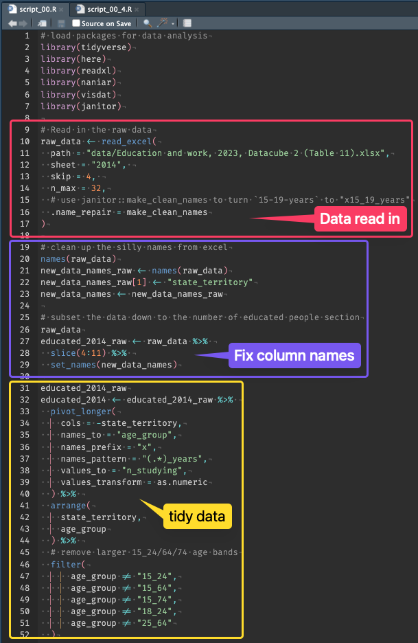
Inside-Out: Breaking code into chunks

50 lines of code
Is not 50 ideas
Chunk code into ideas
Reason with them
Find the complexity
Abstract complexity

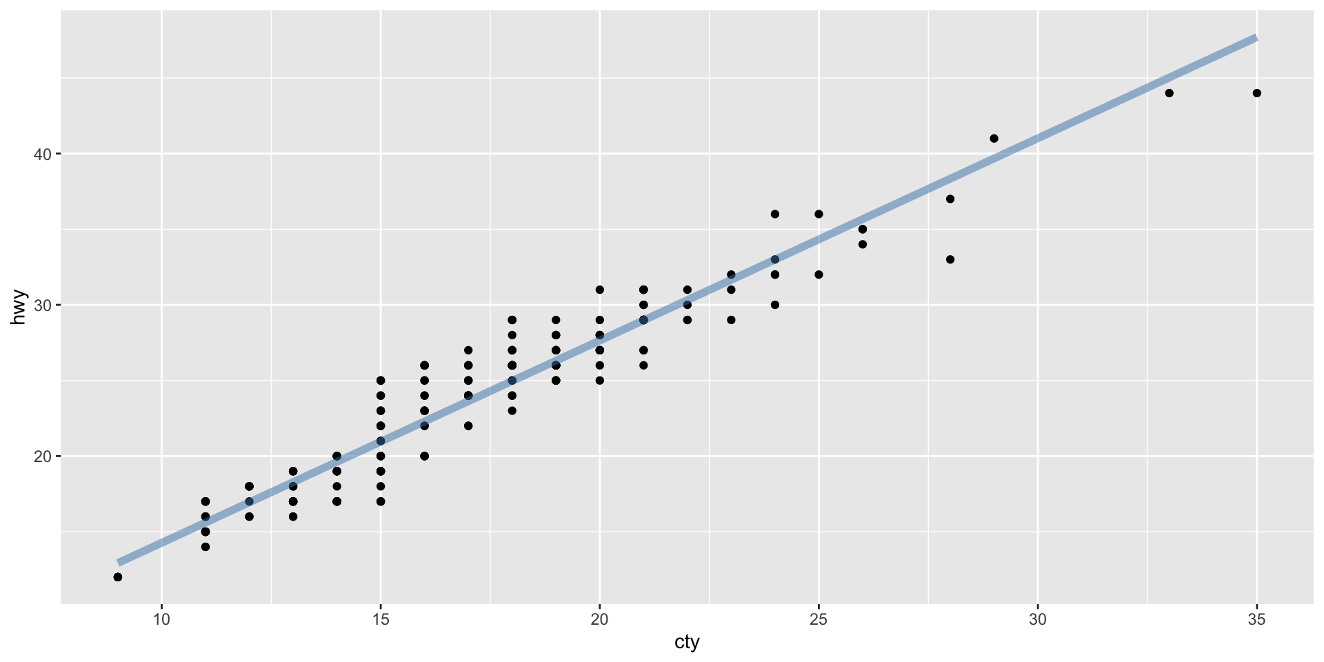
Beware! Abstractions all the way down: ggplot2

Ways to reuse ggplot code

Custom ggplot2 code often involves:

data preparation
aesthetic mappings
multiple custom layers (geom, coord, scale etc.)

Given working ggplot2 code (insides), how might we package this into one or more reusable functions?

Copy & Paste

ggplot(
  data = penguins, 
  mapping = aes(
    x = bill_length_mm,
    y = bill_depth_mm,
    color = species)) +
  geom_point()

## -- SPOT THE DIFFERENCE --

ggplot(
  data = penguins, 
  mapping = aes(
    x = bill_length_mm,
    y = flipper_length_mm,
    color = species)) +
  geom_point()

Store layers as objects or in lists

💡 Useful if components are exactly the same each time!

ggplot(mpg, aes(cty, hwy)) + 
  geom_point() + 
  geom_smooth(
  method = "lm", 
  se = FALSE, 
  colour = alpha("steelblue", 0.5),
  linewidth = 2
)

Store layers as objects or in lists

💡 Useful if components are exactly the same each time!

bestfit <- 
geom_smooth(
  method = "lm", 
  se = FALSE, 
  colour = alpha("steelblue", 0.5),
  linewidth = 2
)
ggplot(mpg, aes(cty, hwy)) + 
  geom_point() + 
  bestfit

Store layers as objects or in functions

geom_mean <- function() {
  list(
    stat_summary(fun = "mean", geom = "bar", fill = "grey70"),
    stat_summary(fun.data = "mean_cl_normal", geom = "errorbar", width = 0.4)
  )
}
ggplot(mpg, aes(class, cty)) + geom_mean()
ggplot(mpg, aes(drv, cty)) + geom_mean()

Helper functions: Convenience vs. flexibility

library(ggweekly)

Error in library(ggweekly): there is no package called 'ggweekly'

ggweek_planner(
  start_day = "2019-04-01", 
  end_day = "2019-06-30", 
)

Error in ggweek_planner(start_day = "2019-04-01", end_day = "2019-06-30", : could not find function "ggweek_planner"

What about customisation?

ggweekly::ggweek_planner(
    start_day = lubridate::today(),
    end_day = start_day +
        lubridate::weeks(8) - lubridate::days(1),
    highlight_days = NULL,
    week_start = c("isoweek", "epiweek"),
    week_start_label = c("month day", "week", "none"),
    show_day_numbers = TRUE,
    show_month_start_day = TRUE,
    show_month_boundaries = TRUE,
    highlight_text_size = 2,
    month_text_size = 4,
    day_number_text_size = 2,
    month_color = "#f78154",
    day_number_color = "grey80",
    weekend_fill = "#f8f8f8",
    holidays = ggweekly::us_federal_holidays,
    font_base_family = "PT Sans",
    font_label_family = "PT Sans Narrow",
    font_label_text = NULL
)

Similar function, different wrapper?

library(ggcal)

Error in library(ggcal): there is no package called 'ggcal'

mydate <- 
  seq(
    as.Date("2017-02-01"),
    as.Date("2017-07-22"),
    by="1 day")
myfills <- 
  rnorm(length(mydate))

print(ggcal(mydate, myfills))

Error in ggcal(mydate, myfills): could not find function "ggcal"

how many arguments does ggcal() have?
what format should dates, fills be?

Another helpful calendar maker?

calendR(
    year = format(Sys.Date(), "%Y"),
    month = NULL,
    from = NULL,
    to = NULL,
    start = c("S", "M"),
    orientation = c("portrait", "landscape"),
    title,
    title.size = 20,
    title.col = "gray30",
    subtitle = "",
    subtitle.size = 10,
    subtitle.col = "gray30",
    text = NULL,
    text.pos = NULL,
    text.size = 4,
    text.col = "gray30",
    special.days = NULL,
    special.col = "gray90",
    gradient = FALSE,
    low.col = "white",
    col = "gray30",
    lwd = 0.5,
    lty = 1,
    font.family = "sans",
    font.style = "plain",
    day.size = 3,
    days.col = "gray30",
    weeknames,
    weeknames.col = "gray30",
    weeknames.size = 4.5,
    week.number = FALSE,
    week.number.col = "gray30",
    week.number.size = 8,
    monthnames,
    months.size = 10,
    months.col = "gray30",
    months.pos = 0.5,
    mbg.col = "white",
    legend.pos = "none",
    legend.title = "",
    bg.col = "white",
    bg.img = "",
    margin = 1,
    ncol,
    lunar = FALSE,
    lunar.col = "gray60",
    lunar.size = 7,
    pdf = FALSE,
    doc_name = "",
    papersize = "A4"
)

Is this using ggplot2?
What are the inputs?
Internal data preparation?
…?

ASIDE: Inspecting Functions

To look at the defintions of your own custom functions:

my_function

To look at functions from packages:

package::function

Over-sized functions?

calendR::calendR

function (year = format(Sys.Date(), "%Y"), month = NULL, from = NULL, 
    to = NULL, start = c("S", "M"), orientation = c("portrait", 
        "landscape"), title, title.size = 20, title.col = "gray30", 
    subtitle = "", subtitle.size = 10, subtitle.col = "gray30", 
    text = NULL, text.pos = NULL, text.size = 4, text.col = "gray30", 
    special.days = NULL, special.col = "gray90", gradient = FALSE, 
    low.col = "white", col = "gray30", lwd = 0.5, lty = 1, font.family = "sans", 
    font.style = "plain", day.size = 3, days.col = "gray30", 
    weeknames, weeknames.col = "gray30", weeknames.size = 4.5, 
    week.number = FALSE, week.number.col = "gray30", week.number.size = 8, 
    monthnames, months.size = 10, months.col = "gray30", months.pos = 0.5, 
    mbg.col = "white", legend.pos = "none", legend.title = "", 
    bg.col = "white", bg.img = "", margin = 1, ncol, lunar = FALSE, 
    lunar.col = "gray60", lunar.size = 7, pdf = FALSE, doc_name = "", 
    papersize = "A4") 
{
    if (year < 0) {
        stop("You must be kidding. You don't need a calendar of a year Before Christ :)")
    }
    wend <- TRUE
    l <- TRUE
    if ((!is.null(from) & is.null(to))) {
        stop("Provide an end date with the 'to' argument")
    }
    if ((is.null(from) & !is.null(to))) {
        stop("Provide a start date with the 'from' argument")
    }
    if (is.character(special.days) & length(unique(na.omit(special.days))) != 
        length(special.col)) {
        stop("The number of colors supplied on 'special.col' argument must be the same of length(unique(na.omit(special.days)))")
    }
    if (length(unique(start)) != 1) {
        start <- "S"
    }
    if (length(unique(orientation)) != 1) {
        orientation <- "landscape"
    }
    if (missing(ncol)) {
        ncol <- ifelse(orientation == "landscape" | orientation == 
            "l", 4, 3)
    }
    match.arg(start, c("S", "M"))
    match.arg(orientation, c("landscape", "portrait", "l", "p"))
    match.arg(papersize, c("A6", "A5", "A4", "A3", "A2", "A1", 
        "A0"))
    if (!is.null(month)) {
        if (month > 12) {
            stop("There are no more than 12 months in a year")
        }
        if (month <= 0) {
            stop("Months must be between 1 and 12")
        }
        if (is.character(month)) {
            stop("You must provide a month in a numeric format, between 1 and 12")
        }
    }
    months <- format(seq(as.Date("2016-01-01"), as.Date("2016-12-01"), 
        by = "1 month"), "%B")
    if (!is.null(text) && is.null(text.pos)) {
        warning("Select the number of days for the text with the 'text.pos' argument")
    }
    if (is.null(text) && !is.null(text.pos)) {
        warning("Add text with the 'text' argument")
    }
    if (missing(weeknames)) {
        up <- function(x) {
            substr(x, 1, 1) <- toupper(substr(x, 1, 1))
            x
        }
        Day <- seq(as.Date("2020-08-23"), by = 1, len = 7)
        weeknames <- c(up(weekdays(Day))[2:7], up(weekdays(Day))[1])
    }
    if (!is.null(from) & !is.null(to)) {
        if (as.numeric(as.Date(from) - as.Date(to)) > 0) {
            stop("'to' must be posterior to 'from'")
        }
        if (lunar == TRUE) {
            l <- FALSE
            warning("Lunar phases are only available for monthly calendars")
        }
        mindate <- as.Date(from)
        maxdate <- as.Date(to)
        weeknames <- substring(weeknames, 1, 3)
    }
    else {
        if (is.null(month)) {
            mindate <- as.Date(format(as.Date(paste0(year, "-0", 
                1, "-01")), "%Y-%m-01"))
            maxdate <- as.Date(format(as.Date(paste0(year, "-12-", 
                31)), "%Y-%m-31"))
            weeknames <- substring(weeknames, 1, 3)
        }
        else {
            if (month >= 10) {
                mindate <- as.Date(format(as.Date(paste0(year, 
                  "-", month, "-01")), "%Y-%m-01"))
            }
            else {
                mindate <- as.Date(format(as.Date(paste0(year, 
                  "-0", month, "-01")), "%Y-%m-01"))
            }
            maxdate <- seq(mindate, length = 2, by = "months")[2] - 
                1
        }
    }
    if (!is.null(from) & !is.null(to)) {
        if (as.Date(to) - as.Date(from) > 366) {
            stop("'from' and 'to' can't me more than 1 year appart")
        }
        if (as.numeric(as.Date(to) - as.Date(from)) > 0) {
            filler <- dplyr::tibble(date = seq(mindate, maxdate, 
                by = "1 day"))
            dates <- seq(mindate, maxdate, by = "1 day")
        }
        else {
            stop("'to' must be posterior to 'from'")
        }
    }
    else {
        filler <- dplyr::tibble(date = seq(mindate, maxdate, 
            by = "1 day"))
        dates <- seq(mindate, maxdate, by = "1 day")
    }
    fills <- numeric(length(dates))
    texts <- character(length(dates))
    texts[text.pos] <- text
    moon_m <- suncalc::getMoonIllumination(date = dates, keep = c("fraction", 
        "phase", "angle"))
    moon <- moon_m[, 2]
    right <- ifelse(moon_m[, 4] < 0, TRUE, FALSE)
    if (is.character(special.days)) {
        if (length(special.days) != length(dates)) {
            if (special.days != "weekend") {
                stop("special.days must be a numeric vector, a character vector of the length of the number of days of the year or month or 'weekend'")
            }
            else {
                wend <- FALSE
            }
        }
        if (gradient == TRUE) {
            warning("Gradient won't be created as 'special.days' is of type character. Set gradient = FALSE in this scenario to avoid this warning")
            if (legend.title != "" & legend.pos == "none") {
                warning("Legend title specified, but legend.pos == 'none', so no legend will be plotted")
            }
        }
        else {
            if (length(special.days) != length(dates) & (legend.pos != 
                "none" | legend.title != "")) {
                legend.pos = "none"
                warning("gradient = FALSE, so no legend will be plotted")
            }
        }
    }
    else {
        if (gradient == FALSE) {
            if (length(special.days) != length(dates) & (legend.pos != 
                "none" | legend.title != "")) {
                legend.pos = "none"
                warning("gradient = FALSE, so no legend will be plotted")
            }
        }
        else {
            if (legend.title != "" & legend.pos == "none") {
                warning("Legend title specified, but legend.pos == 'none', so no legend will be plotted")
            }
        }
        if (gradient == TRUE & (length(special.days) != length(dates))) {
            stop("If gradient = TRUE, the length of 'special.days' must be the same as the number of days of the corresponding month or year")
        }
    }
    if (start == "M") {
        weekdays <- weeknames
        t1 <- dplyr::tibble(date = dates, fill = fills) %>% right_join(filler, 
            by = "date") %>% mutate(dow = ifelse(as.numeric(format(date, 
            "%w")) == 0, 6, as.numeric(format(date, "%w")) - 
            1)) %>% mutate(month = format(date, "%B")) %>% mutate(woy = as.numeric(format(date, 
            "%W"))) %>% mutate(year = as.numeric(format(date, 
            "%Y"))) %>% mutate(month = toupper(factor(month, 
            levels = months, ordered = TRUE))) %>% mutate(monlabel = month)
        if (!is.null(month)) {
            t1$monlabel <- paste(t1$month, t1$year)
        }
        t2 <- t1 %>% mutate(monlabel = factor(monlabel, ordered = TRUE)) %>% 
            mutate(monlabel = fct_inorder(monlabel)) %>% mutate(monthweek = woy - 
            min(woy), y = max(monthweek) - monthweek + 1) %>% 
            mutate(weekend = ifelse(dow == 6 | dow == 5, 1, 0))
        if (all(special.days == 0) == TRUE || length(special.days) == 
            0) {
            special.col <- "white"
        }
        else {
            if (is.character(special.days)) {
                if (length(special.days) == length(dates)) {
                  fills <- special.days
                }
                else {
                  if (special.days == "weekend") {
                    fills <- t2$weekend
                  }
                }
            }
            else {
                if (gradient == TRUE) {
                  fills <- special.days
                }
                else {
                  fills[special.days] <- 1
                }
            }
        }
    }
    else {
        weekdays <- c(weeknames[7], weeknames[1:6])
        t1 <- dplyr::tibble(date = dates, fill = fills) %>% right_join(filler, 
            by = "date") %>% mutate(dow = as.numeric(format(date, 
            "%w"))) %>% mutate(month = format(date, "%B")) %>% 
            mutate(woy = as.numeric(format(date, "%U"))) %>% 
            mutate(year = as.numeric(format(date, "%Y"))) %>% 
            mutate(month = toupper(factor(month, levels = months, 
                ordered = TRUE))) %>% mutate(monlabel = month)
        if (!is.null(month)) {
            t1$monlabel <- paste(t1$month, t1$year)
        }
        t2 <- t1 %>% mutate(monlabel = factor(monlabel, ordered = TRUE)) %>% 
            mutate(monlabel = fct_inorder(monlabel)) %>% mutate(monthweek = woy - 
            min(woy), y = max(monthweek) - monthweek + 1) %>% 
            mutate(weekend = ifelse(dow == 0 | dow == 6, 1, 0))
        if (all(special.days == 0) == TRUE || length(special.days) == 
            0) {
            special.col <- "white"
        }
        else {
            if (is.character(special.days)) {
                if (length(special.days) == length(dates)) {
                  fills <- special.days
                }
                else {
                  if (special.days == "weekend") {
                    fills <- t2$weekend
                  }
                }
            }
            else {
                if (gradient == TRUE) {
                  fills <- special.days
                }
                else {
                  fills[special.days] <- 1
                }
            }
        }
    }
    df <- data.frame(week = weekdays, pos.x = 0:6, pos.y = rep(max(t2$monthweek) + 
        1.75, 7))
    if (missing(title)) {
        if (!is.null(from) & !is.null(to)) {
            title <- paste0(format(as.Date(from), "%m"), "/", 
                format(as.Date(from), "%Y"), " - ", format(as.Date(to), 
                  "%m"), "/", format(as.Date(to), "%Y"))
        }
        else {
            if (is.null(month)) {
                title <- year
            }
            else {
                title <- levels(t2$monlabel)
            }
        }
    }
    if (week.number == FALSE) {
        week.number.col <- "transparent"
    }
    if (is.null(month) | (!is.null(from) & !is.null(to))) {
        if (!missing(monthnames)) {
            if (length(monthnames) == length(levels(t2$monlabel))) {
                t2$monlabel <- factor(t2$monlabel, labels = monthnames)
            }
            else {
                stop("The length of 'monthname's must equal to the number months")
            }
        }
        if (lunar == TRUE & l != FALSE) {
            warning("Lunar phases are only available for monthly calendars")
        }
        if (gradient == TRUE || !missing(special.days)) {
            p <- ggplot(t2, aes(dow, woy + 1)) + geom_tile(aes(fill = fills), 
                color = col, size = lwd, linetype = lty)
        }
        else {
            p <- ggplot(t2, aes(dow, woy + 1)) + geom_tile(aes(fill = fills), 
                fill = low.col, color = col, size = lwd, linetype = lty)
        }
        if (is.null(from) & is.null(to)) {
            weeklabels <- 1:53
            if (length(t2$date) == 365) {
                weeklabels <- 1:53
            }
            else {
                if (t2$dow[1] == 6) {
                  weeklabels <- 1:54
                }
            }
        }
        else {
            weeklabels <- unique(t2$woy) + 1
        }
        if (is.character(special.days) & wend & length(unique(special.days) == 
            length(dates))) {
            p <- p + scale_fill_manual(values = special.col, 
                labels = levels(as.factor(fills)), na.value = "white", 
                na.translate = FALSE)
        }
        else {
            p <- p + scale_fill_gradient(low = low.col, high = special.col, 
                na.value = "white")
        }
        p <- p + facet_wrap(~monlabel, ncol = ncol, scales = "free") + 
            ggtitle(title) + labs(subtitle = subtitle) + scale_x_continuous(expand = c(0.01, 
            0.01), position = "top", breaks = seq(0, 6), labels = weekdays) + 
            scale_y_continuous(expand = c(0.01, 0.01), trans = "reverse", 
                breaks = unique(t2$woy) + 1, labels = weeklabels) + 
            geom_text(data = t2, aes(label = gsub("^0+", "", 
                format(date, "%d"))), size = day.size, family = font.family, 
                color = days.col, fontface = font.style) + labs(fill = legend.title) + 
            theme(panel.background = element_rect(fill = NA, 
                color = NA), strip.background = element_rect(fill = mbg.col, 
                color = mbg.col), plot.background = element_rect(fill = bg.col), 
                panel.grid = element_line(colour = ifelse(bg.img == 
                  "", bg.col, "transparent")), strip.text.x = element_text(hjust = months.pos, 
                  face = font.style, color = months.col, size = months.size), 
                legend.title = element_text(), axis.ticks = element_blank(), 
                axis.title = element_blank(), axis.text.y = element_text(colour = week.number.col, 
                  size = week.number.size), axis.text.x = element_text(colour = weeknames.col, 
                  size = weeknames.size * 2.25), plot.title = element_text(hjust = 0.5, 
                  size = title.size, colour = title.col), plot.subtitle = element_text(hjust = 0.5, 
                  face = "italic", colour = subtitle.col, size = subtitle.size), 
                legend.position = legend.pos, plot.margin = unit(c(1 * 
                  margin, 0.5 * margin, 1 * margin, 0.5 * margin), 
                  "cm"), text = element_text(family = font.family, 
                  face = font.style), strip.placement = "outsite")
        if (bg.img != "") {
            p <- ggbackground(p, bg.img)
        }
    }
    else {
        tidymoons <- data.frame(x = t2$dow + 0.35, y = t2$y + 
            0.3, ratio = moon, right = right)
        tidymoons2 <- data.frame(x = t2$dow + 0.35, y = t2$y + 
            0.3, ratio = 1 - moon, right = !right)
        p <- ggplot(t2, aes(dow, y)) + geom_tile(aes(fill = fills), 
            color = col, size = lwd, linetype = lty)
        if (lunar == TRUE) {
            p <- p + geom_moon(data = tidymoons, aes(x, y, ratio = ratio, 
                right = right), size = lunar.size, fill = "white") + 
                geom_moon(data = tidymoons2, aes(x, y, ratio = ratio, 
                  right = right), size = lunar.size, fill = lunar.col)
        }
        if (is.character(special.days) & wend & length(unique(special.days) == 
            length(dates))) {
            p <- p + scale_fill_manual(values = special.col, 
                labels = levels(as.factor(fills)), na.value = "white", 
                na.translate = FALSE)
        }
        else {
            p <- p + scale_fill_gradient(low = low.col, high = special.col, 
                na.value = "white")
        }
        p <- p + ggtitle(title) + labs(subtitle = subtitle) + 
            geom_text(data = df, aes(label = week, x = pos.x, 
                y = pos.y), size = weeknames.size, family = font.family, 
                color = weeknames.col, fontface = font.style) + 
            geom_text(aes(label = texts), color = text.col, size = text.size, 
                family = font.family) + scale_y_continuous(expand = c(0.05, 
            0.05), labels = rev(unique(t2$woy)), breaks = 1:length(unique(t2$woy))) + 
            geom_text(data = t2, aes(label = 1:nrow(filler), 
                x = dow - 0.4, y = y + 0.35), size = day.size, 
                family = font.family, color = days.col, fontface = font.style) + 
            labs(fill = legend.title) + theme(panel.background = element_rect(fill = NA, 
            color = NA), strip.background = element_rect(fill = NA, 
            color = NA), plot.background = element_rect(fill = bg.col), 
            panel.grid = element_line(colour = ifelse(bg.img == 
                "", bg.col, "transparent")), strip.text.x = element_text(hjust = 0, 
                face = "bold", size = months.size), legend.title = element_text(), 
            axis.ticks = element_blank(), axis.title = element_blank(), 
            axis.text.y = element_text(colour = week.number.col, 
                size = week.number.size), axis.text.x = element_blank(), 
            plot.title = element_text(hjust = 0.5, size = title.size, 
                colour = title.col), plot.subtitle = element_text(hjust = 0.5, 
                face = "italic", colour = subtitle.col, size = subtitle.size), 
            legend.position = legend.pos, plot.margin = unit(c(1 * 
                margin, 0.5 * margin, 1 * margin, 0.5 * margin), 
                "cm"), text = element_text(family = font.family, 
                face = font.style), strip.placement = "outsite")
        if (bg.img != "") {
            p <- ggbackground(p, bg.img)
        }
    }
    if (pdf == FALSE & doc_name != "") {
        warning("Set pdf = TRUE to save the current calendar")
    }
    if (pdf == TRUE) {
        switch(papersize, A6 = {
            a <- 148
            b <- 105
        }, A5 = {
            a <- 210
            b <- 148
        }, A4 = {
            a <- 297
            b <- 210
        }, A3 = {
            a <- 420
            b <- 297
        }, A2 = {
            a <- 594
            b <- 420
        }, A1 = {
            a <- 841
            b <- 594
        }, A0 = {
            a <- 1189
            b <- 841
        }, )
        if (doc_name == "") {
            if (!is.null(month)) {
                doc_name <- paste0("Calendar_", tolower(t2$month[1]), 
                  "_", year, ".pdf")
            }
            else {
                if (!is.null(from) & !is.null(to)) {
                  doc_name <- paste0("Calendar_", from, "_", 
                    to, ".pdf")
                }
                else {
                  doc_name <- paste0("Calendar_", year, ".pdf")
                }
            }
        }
        else {
            doc_name <- paste0(doc_name, ".pdf")
        }
        if (orientation == "landscape" | orientation == "l") {
            ggsave(filename = if (!file.exists(doc_name)) 
                doc_name
            else stop("File does already exist!"), height = b, 
                width = a, units = "mm")
        }
        else {
            ggsave(filename = if (!file.exists(doc_name)) 
                doc_name
            else stop("File does already exist!"), width = b, 
                height = a, units = "mm")
        }
    }
    return(p)
}
<bytecode: 0xa87c7ef58>
<environment: namespace:calendR>

Beware false savings!

Sometimes

“saved” lines of code

turn into

confusing lists of plot specific arguments

Summary

Functions in R

How to write valid functions
How to test functions
How to break down data analysis workflows into smaller tasks (or functions)
Style considerations for function names, errors and interfaces
Strategies for designing better functions

Strategies for DRRY functions

Outside in:

Name: What am I trying to do? What evokes the action
Inputs: What pieces of information do I need to provide?
Output: What are we returning?

Inside out:

Copy text into body
Identify complexity to manage
Abstract the complexity

Advanced Statistical Programming using R

Reminders

Contact Us

Last Week

Reviewing RStudio with the Knife / Kitchen analogy

Command Line

Git for version history

Why command line git?

This Week

Individual Reflection Log

Review: Writing Functions

What are functions?

Defining a function in R

Function syntax in R

Testing Functions

Why test functions?

Testing Sensible Inputs

Stress-testing functions

Validating Function inputs

When testing is hard

Matters of design & style

Things to consider when writing a function…

Naming functions (as verbs)

Extension: Documenting (package) functions

Writing better error messages

Extension: Better errors with cli

Avoid writing greedy functions

What granularity? Task abstractions

What granularity? Task abstractions

Writing (better) functions

Why write (better) functions?

Moving beyond DRY (Don’t Repeat Yourself)

Writing DRRY functions

Outside to Inside and Back again

Outside-in: Principles

Outside-in: Context

Outside-in: Naming

Inside-Out: Breaking code into chunks

Beware! Abstractions all the way down: ggplot2

Ways to reuse ggplot code

Copy & Paste

Store layers as objects or in lists

Store layers as objects or in lists

Store layers as objects or in functions

Helper functions: Convenience vs. flexibility

Similar function, different wrapper?

Another helpful calendar maker?

ASIDE: Inspecting Functions

Over-sized functions?

Beware false savings!

Summary

Functions in R

Strategies for DRRY functions

Extension: Better errors with `cli`