Rows: 5
Columns: 4
$ id <dbl> 1, 2, 3, 4, 5
$ date <chr> "3/1/10", "3/2/10", "3/3/10", "3/4/10", "3/5/10"
$ loc <chr> "New York", "New York", "New York", "New York", "New York"
$ temp <dbl> 42.0, 41.4, 38.5, 41.1, 39.8Advanced Statistical Programming using R
Week 7: Initial Data Analysis & Data Cleaning
2026-05-28
Announcements
Reminders
- All groups should be registered:
- Group member names & LMU campus emails
- GitHub repo (set up this week in lecture/practical)
- Proposal submission deadline extended to start of W8 (Mon Jun 8)
- Review the project guidelines
- Set up your project repository structure
- Include a proposal document & start drafting based on project proposal guidelines
- Submission will be via a separate Moodle form.
Pick your datasets by tomorrow (May 29)!
This week’s practical will be based around helping you prepare your group project proposals. The practical will be most helpful if you have collected the data you plan to use in your projects.
Tips
Projects must be based on a cohesive set of data (i.e. your dataset), in a single GitHub repo, and available on the web. It is intended to help you gain hands-on experience with statistical programming skills.
If you don’t know where to start, try:
- Turning code for data import, cleaning, or tidying into functions — and collecting them into an R package
- Putting visualisations into different layouts on a Quarto webpage
- Describing how the dataset was collected and what it contains (variables, rows, licence)
- Documenting discussions — e.g. “We wanted to look at daily temperatures vs. museum visitors, but visitor numbers were only monthly, so we instead explored…”
FAQs
Q: What format is the project?
A: Up to you! Be creative.
Q: Do we have to use a particular dataset?
A: No — any openly licensed data source is fine.
Q: Can we work in groups of 2? or alone?
A: Yes, though 3–4 is recommended so you have more chances to encounter merge conflicts and manage pull requests.
Suggestions for Final Output
The format should suit your analysis context and target audience:
- Statistical report — e.g. ModernDive example
- Collection of charts — e.g. VisTales example
- Interactive dashboard — using the Quarto Dashboards format
- Data storytelling article — using the Closeread extension
- R Data Package with pkgdown website — e.g. palmerpenguins
Key dates
| Milestone | Date | Submission |
|---|---|---|
| May 22 | Group members, GitHub repo URL | |
| Proposal | Start in W7 practical, due 8 Jun | URL to rendered proposal |
| Group reflection — in-class discussion | W14 practical | N/A |
Final submission + group-reflection.qmd |
Due 22 Jul | URL to final website/webpage, group reflection doc |
| Individual contribution statement | Due 23 Jul | PDF via Moodle |
| Oral exam | 29 Jul | — |
Submission Formats
- All submissions will be via forms on Moodle.
- The final submission should be a URL to a rendered website.
- The
group-reflection.qmddocuments what your group did, how you used LLMs, and key decisions contribution.pdfdocuments your contribution to your group project, and the specific tasks and skills you worked on.- For anyone working alone (i.e. groups of 1), your group reflection & contribution statements can be the same.
Relation to Oral Exam
Students who submit individual contribution statements will have oral exam questions related to their own work. Otherwise, the oral exam questions will involve generic projects.
Syllabus
Syllabus
Part 1: Statistical Programming Foundations
- W02: Scripts, Functions & Refactoring
- W03: Debugging
- W04: Version Control & Remotes
- W05: Quarto Websites & Collaborative Coding
- W06: R Packages
Part 2: Working with Real World Data
- W07: Initial Data Analysis & Data Cleaning
- W09: Open Data & Renv
- W10: Modelling & Analysis
- W11: Statistical Communication & Visualisation
Part 3: Advanced Topics & Summary
- W12: Interactive Data Storytelling
- W13: Multi-lingual Analysis (Python/R)
- W14: Review & Outro
Last Week
R Packages
- A package is the standard unit for sharing functions, data, and documentation in R
usethis&devtoolsstreamline the development workflow: create → document → check → install- Data packages (e.g.
munichvisitors) distribute clean, documented datasets — a great first package roxygen2turns#'comments into.Rdhelp files — document as you write
Documentation & Design
- Every exported object needs
@param,@returns,@export, and@examples - Expose data as an argument (
data = museum_visitors) when users may want to filter or swap it - Single responsibility — each function does one thing; package groups functions with a shared theme
- Consistent interfaces —
datafirst, options last with sensible defaults - Limit dependencies — every imported package is a liability your users inherit
This Week
- Initial Data Analysis
- Data Screening
- Data Cleaning
- Missing Data
Initial Data Analysis
Based on: https://ddde.numbat.space/week3/slides.html#/title-slide, Huebner et al. (2018), Huebner et al. (2020)
Idealised Statistical Investigation
From Chatfield (1985):
- Clarify the objectives of the investigation
- Collect the data in an appropriate way
- Investigate the structure and quality of the data
- Carry out an initial examination of the data
- Select and carry out an appropriate formal statistical analysis
- Compare findings with previous results or acquire further data
- Interpret and communicate the results
Note
Steps 3 & 4 describe Initial Data Analysis (IDA).
What is Initial Data Analysis?
“IDA is a systematic and documented pre-analysis examination of a dataset, carried out before formal statistical analysis and without reference to the main research questions.” — adapted from Huebner et al. (2018)
Where does IDA fit?
- Occurs between data collection and planned statistical analyses
- Does not touch the research questions
What does IDA uncover?
- Missing values
- Subgroups with small sample sizes
- Data collection shortcomings
- Impact of these issues on research results
IDA, EDA, and CDA
Exploratory Data Analysis
- Hypothesis-generating
- Open-ended exploration
- May shift research direction
Confirmatory Data Analysis
- Executes the statistical analysis plan (SAP)
- Answers predefined research questions
Initial Data Analysis
- Ensures transparency & integrity
- Checks preconditions for analysis
- Does not directly answer research questions
Shared methods and tools
All three types of analysis use statistical visualisation and summaries. The difference is intent and timing, not technique.
IDA vs EDA vs CDA
| IDA | EDA | CDA | |
|---|---|---|---|
| Goal | Check preconditions; ensure data integrity | Generate hypotheses | Answer predefined research questions |
| Scope | Systematic, pre-specified | Open-ended | Planned (statistical analysis plan) |
| Relation to research questions | Must not touch them | May reshape them | Answers them |
| When | Before analysis begins | Early–mid analysis | After IDA + EDA |
| Output | Documentation of data issues & decisions | New hypotheses, patterns | Statistical inference, conclusions |
Relation to Data Science Workflow
From R4DS:
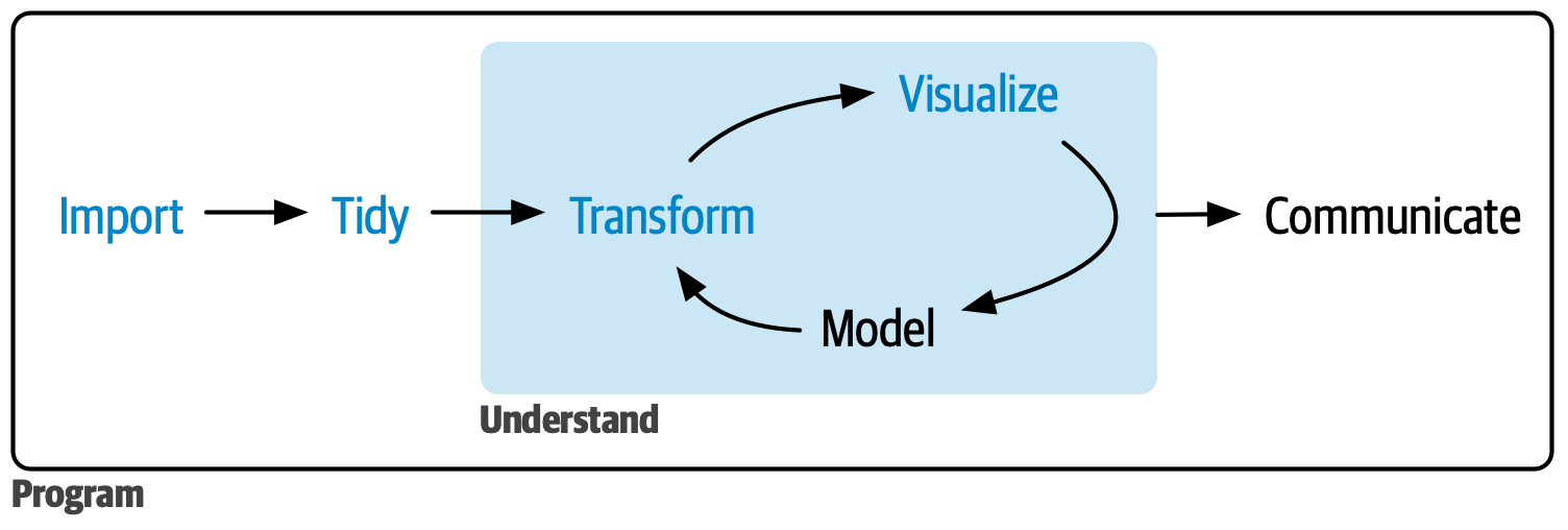
- Statistical analysis involves both planned (sequential) and exploratory (iterative) phases and subphases.
- IDA maps most easily to import, tidy & transform stages
- But IDA investigations may also involve all components of a data science workflow:
- e.g. using visualisation to identify data quality issues
IDA in practice
Guiding principle
IDA strategies require careful thinking and design based on problem and context, not analyst preference.
“There are no routine statistical questions, only questionable statistical routines.” — David R. Cox
- Reporting is mixed and varied across data analysis reports and research papers
- Part of the statistical value chain in official statistics
- A skill developed through practice and hands-on reasoning about data
- Forces you to engage with assumptions you might unconsciously make about data
Uncovering data issues in IDA
Issues found during IDA can occur at multiple levels:
- Univariate — problems within a single variable (wrong type, outliers, unexpected distribution)
- Multivariate — problems across variables (unexpected correlations, group imbalances, distributional differences by subgroup)
- Dataset — structural problems (missing rows, duplicate observations, wrong unit of analysis)
IDA & the Analysis Plan
Issues uncovered during IDA may require updating the statistical analysis plan before proceeding to CDA.
| Topic | Examples | Possible influence on Analysis Plan |
|---|---|---|
| Suspicious values | Outliers; inconsistent follow-up dates; conflicting diagnosis sources | Rules for whether/how to use inconsistent information |
| Suspicious subjects | Doubts on inclusion criteria; highly corrupt subject data | Exclusion decisions balancing data cleanliness vs. selection bias |
| Unexpected heterogeneity | Incompatible education systems; centre-level measurement differences | Exclusion or stratification; re-examining measurement instructions |
| Variable distribution | Unexpectedly skewed covariates; bimodal continuous variables | Transformations; splitting variables; adapting statistical methods |
| Violated method requirements | Non-normal outcomes; asymptotic tests with small subgroups | Refinement, extension, or reduction of models |
IDA and Inference
The Goal of IDA: is to avoid misleading or inappropriate statistical analyses. However, IDA can compromise validity of inference if you:
- Change inference or research questions based on IDA findings
- Make undocumented or unjustified decisions about:
- Outlier removal or retention
- Missing value imputation strategy
- Treatment of zeros
- Variable type handling (categorical, temporal)
- Variable and observation selection
- Skip multivariate relationship checks or subgroup-level checks
Protecting CDA validity after IDA
Justify key decisions
- Outlier removal or retention
- Variable selection & recoding
- Sampling choices
- Handling of zeros
Document everything
- Record ALL IDA in a reproducible analysis script
- Pre-register your CDA plan so research questions cannot drift — ensures against accusations of data snooping, data dredging, or data fishing.
IDA in StatProg2
We cover IDA across several weeks — each builds on the last:
| IDA component | When |
|---|---|
| Data screening — checking types, context, distributions | W7 (this lecture) |
| Data cleaning / preprocessing — fixing issues found in screening | W7 (this lecture + practical) |
| Analysis planning & updating — refining the analysis plan based on IDA findings | W7 practical + W10 |
| Reporting & documentation — recording IDA decisions reproducibly | W9 (next lecture) |
Group project
Your project proposal should include both an IDA plan (what you will screen and clean) and a CDA plan (the research questions you will answer). IDA findings may lead you to refine your CDA plan before analysis.
Review: Data Import & Tidying
- getting data into R
- tidying and reshaping data
Reading data into R
| Format | Function | Package |
|---|---|---|
| CSV / TSV | read_csv(), read_tsv() |
readr |
| Excel (.xlsx, .xls) | read_excel() |
readxl |
| SPSS / Stata / SAS | read_sav(), read_dta(), read_sas() |
haven |
| JSON | fromJSON() |
jsonlite |
| Parquet | read_parquet() |
arrow |
| Database | dbReadTable(), tbl() |
DBI / dbplyr |
Tip
Prefer readr::read_csv() over base read.csv() — it produces a tibble, infers column types with explicit feedback, and is faster on large files.
Raw, Interim & Final Data
Folder convention
data/raw/— original source files; never modifieddata/interim/— intermediate.rdssnapshots from cleaning scriptsdata/final/— analysis-ready dataset; reproducibly derived fromraw/
my-project/
├── data/
│   ├── raw/          ← source files; read-only
│   ├── interim/      ← .rds cleaning snapshots
│   └── final/        ← analysis-ready dataset
├── code/
│   ├── 01-import.R
│   ├── 02-clean.R
│   └── 03-analyse.R
├── docs/
└── my-project.Rproj
Importing and caching
Raw data files (Excel, SPSS, database exports) can be slow to re-import. Tidied or cleaned intermediates are often saved as .rds snapshots in data/interim/ rather than re-derived each run.
Import, process and cache
RDS preserves R data types (factors, dates, ordered levels) without re-parsing, unlike saving back to CSV.
Tip
Never overwrite the original raw data file. Save processed versions separately. Write final datasets to common formats like CSV for easier sharing.
Tidy data
Three rules (Wickham, 2014)
- Each variable is a column
- Each observation is a row
- Each value is a single cell
Tidy data is the target state — raw data almost never arrives this way.
Why it matters
- Tidyverse tools (
dplyr,ggplot2,tidyr) assume tidy input - Tidy data makes vectorised operations natural and pipe-friendly
- A shared standard means collaborators can read your data without explanation
Tidying vs. IDA & Cleaning
Tidying is not the same as cleaning — a dataset can be tidy but still have wrong values, bad types, or missing data.
Common tidying tools
| Task | Function | Package |
|---|---|---|
| Standardise column names | clean_names() |
janitor |
| Tabulate a categorical variable | tabyl() |
janitor |
| Reshape wide → long | pivot_longer() |
tidyr |
| Reshape long → wide | pivot_wider() |
tidyr |
| Fill implicit gaps in time series | complete() |
tidyr |
| Recode / transform variables | mutate() |
dplyr |
| Remove duplicate rows | distinct() |
dplyr |
| Filter to valid rows | filter() |
dplyr |
Tip
janitor::clean_names() should almost always be the first step after import — it converts AUSPRAEGUNG → auspraegung, removing spaces and special characters so column names are pipe-safe.
Data screening
- making sure data are represented correctly in R
- identifying data type and format errors
- preliminary characterisation of dataset
Data types & formats
- Data types are semantic vectors — they encode the kind of data, not just its storage
- Basic R types (review):
logical,integer,double,character,factor - Complex types built on top:
Date/POSIXcton numerics;factoron integers
- Basic R types (review):
- Data formats describe how data is encoded on disk
- Some types need specialist import handling (geospatial, images, nested JSON)
Best Practices
Declare types explicitly with col_types when importing, then verify with glimpse(). The R data type should closely match the real-world meaning of the variable.
Example: New York Temperatures
new-york-temp.csv
id,date,loc,temp
1,3/1/10,New York,42
2,3/2/10,New York,41.4
3,3/3/10,New York,38.5
4,3/4/10,New York,41.1
5,3/5/10,New York,39.8
Checking data types
What happens if you don’t check?
What column types do we get when reading in the New York temperature data?
# A tibble: 5 × 4
     id date   loc       temp
  <dbl> <chr>  <chr>    <dbl>
1     1 3/1/10 New York  42
2     2 3/2/10 New York  41.4
3     3 3/3/10 New York  38.5
4     4 3/4/10 New York  41.1
5 5 3/5/10 New York 39.8- What problems are there with R’s interpretation of the data type?
- What context-specific factors suggest an incorrect interpretation?
Compare with .xlsx import:
# A tibble: 5 × 4
     id date                loc       temp
  <dbl> <dttm>              <chr>    <dbl>
1     1 2010-01-03 00:00:00 New York  42
2     2 2010-02-03 00:00:00 New York  41.4
3     3 2010-03-03 00:00:00 New York  38.5
4     4 2010-04-03 00:00:00 New York  41.1
5 5 2010-05-03 00:00:00 New York 39.8- Excel files carry column type metadata — so
read_excel()can inferdatetime. - CSV is plain text with no type information —
read_csv()must guess, and guesseschrfor ambiguous strings like"1/3/2010". - R has no way to know it is a date without being told.
Fixing data types
library(lubridate)
library(dplyr)

# Step 1: set raw storage type on import
df <- read_excel("data/date-example.xlsx",
                 col_types = c("text",    # id
                               "date",    # date → POSIXct
                               "text",    # loc
                               "numeric"))# temp

# Step 2: convert to intended R types; extract date components
df |>
  mutate(id   = as.factor(id),  # chr → factor
         date = ydm(date)) |>   # POSIXct → Date (year-day-month)
  mutate(day   = day(date),
         month = month(date),
         year  = year(date))
# A tibble: 5 × 7
id date loc temp day month year
<fct> <date> <chr> <dbl> <int> <dbl> <dbl>
1 1 2010-03-01 New York 42 1 3 2010
2 2 2010-03-02 New York 41.4 2 3 2010
3 3 2010-03-03 New York 38.5 3 3 2010
4 4 2010-03-04 New York 41.1 4 3 2010
5 5 2010-03-05 New York 39.8 5 3 2010idis now afactorinstead ofintegerday,month,yearextracted fromdate- Is the data screening issue fixed now?
Ambiguity in Date Formats!
- There are multiple different date formats in widespread usage:
- MM/DD/YYYY (US)
- DD/MM/YYYY (international)
- YYYY/MM/DD (ISO 8601)
- What’s the most likely format in this example?
- Most likely 1st–5th March, not 3rd of Jan–May
- Could check against some reference facts (e.g. look up weather history for New York)
Working with dates in R {lubridate}
Lubridate is a package designed to make working with dates smoother and easier in R.
Parse dates from strings
Tip
Other special data types have dedicated helper packages — e.g. sf for geospatial data, hms for time-of-day, forcats for factors.
Specifying types explicitly
Explicit types catch data errors before they silently affect analysis — a misread date or factor-stored-as-number can corrupt results without any warning.
read_excel() with col_types
Dataset Definition and Quality
Defining and constructing datasets
Dataset conceptualisation is the process of deciding what a dataset should contain before assessing what it does contain.
- What is the unit of observation?
- What is the target population?
- What time period does it cover?
- What variables are required for the analysis?
Why it matters
You cannot assess whether data is complete, suitable, or correctly structured without first defining what the dataset should look like.
The same raw data can produce very different datasets depending on the conceptualisation — e.g. one row per museum visit vs. one row per museum per month.
What is data quality?
Data quality depends on both the dataset itself and the intended use — a dataset can be high quality for one purpose and unsuitable for another.
Context-independent quality
- Is it well documented? (codebook, variable descriptions)
- Are values internally consistent?
- Is the target population and sampling frame clearly defined?
Context-specific quality
- Is the dataset suitable for this analysis task?
- Were appropriate collection methods used for this research question?
- Does the sample represent the population of interest?
Data Cleaning
- investigating
- modifying and fixing
What is data cleaning?
No universal definition
- Data cleaning is commonly used to refer to a variety of data tasks performed before modelling or inference on data.
- Also called data preparation, data preprocessing, or data wrangling
- Think in terms of “preparation” or “preprocessing” to avoid assuming there is one “true clean” version of a dataset
What it involves
- Investigating possible data quality issues
- Making decisions about outliers, missing values, and variable types
- Performed in the context of particular target dataset concept
- Can overlap with ‘data screening’ — there’s no hard rule for which stage you can or will spot certain issues with the data
Data screening, tidying and cleaning
Compared to data screening and tidying, data cleaning requires more judgement and iterative investigation — the tools and methods used depend on what problems are actually found in the data.
Issues within and across variables
Check for issues within individual variables or across the whole dataset:
Variable-level issues
- Values outside plausible range (e.g. negative heights, temperatures above 100°C)
- Non-integer counts; compositional values that don’t sum to 1
- Wrong data type (e.g. date stored as text)
- Missing values (
NA): unrecorded, censored, or not applicable - Skewed, bimodal, or otherwise unexpected distributions
- Detect with:
glimpse(),summary(), histograms, boxplots
Structural / cross-variable issues
- Imbalanced groups (e.g. treatment vs. control demographics differ)
- Train/test distribution mismatch
- Insufficient data at levels of a categorical variable
- CDA assumption violations: non-normality, unequal variance, unexpected discreteness
- Detect with: cross-tabulations, group comparisons, scatter plots
Approaches to identifying issues
Both variable-level and structural / cross-variable issues (see previous section) can be detected with a mix of numerical and graphical tools.
Look at your data
- Eyeballing raw values — catches obvious entry errors and formatting problems
- Numerical summaries:
summary(),skimr::skim() - Graphical summaries: histograms, boxplots, scatter plots
Prioritise graphical checks
- Distributions are easier to read as plots than as tables
- Relationships between variables may only be visible visually
Look and then look again at your data!
Always plot your data before, after and between preparation steps. Exactly what to plot depends on what you are trying to see.
Fixing identified issues
Variable-level fixes
- Recode wrong types:
mutate()+as.*() - Replace or flag out-of-range values
- Standardise inconsistent encodings (e.g.
"M"/"Male"→ consistent factor) - Handle missing values: drop, impute, or flag
Structural fixes
- Remove duplicate rows:
distinct() - Fill implicitly missing rows:
tidyr::complete() - Correct unit of analysis: reshape with
pivot_*() - Split or merge variables:
separate(),unite()
Handling missing values
Can you just drop missing values?
Common practice: drop rows with NA using na.omit() or filter(!is.na(x))
Pitfalls:
- Reduces sample size and statistical power
- May introduce selection bias if values are not missing at random
- Silently changes the population your analysis represents
Warning
Most R functions silently drop NA with na.rm = TRUE — this hides the problem rather than resolving it.
Why missingness is conceptually hard
- The absence of a value is itself informative
- You cannot directly observe why a value is missing
- The right approach depends on the missing data mechanism — not just the proportion missing
Explicit vs. Implicit Missingness
Explicit missingness
NAvalues present in the data- Identified with
is.na(),summary(), ornaniar::vis_miss() - Need to decide: remove, impute, or model the missingness mechanism
Implicit missingness
- Rows that should exist are absent entirely
- Common in longitudinal/time-series data (missing time points) or categorical combinations that were never recorded
- Harder to detect — requires domain knowledge about expected structure
Tools for missingness
naniar — tidy missing data tools
Example: Olympic medals
Explicit NAs are relatively easy to detect — but implicit missingness often requires reasoning about what rows should exist.
             country totalmedal
1       UnitedStates        104
2              China         88
3             Russia         82
4       GreatBritain         65
5            Germany         44
6              Japan         38
7          Australia         35
8             France         34
9         SouthKorea         28
10             Italy         28
11       Netherlands         20
12           Ukraine         20
13            Canada         18
14           Hungary         17
15             Spain         17
16            Brazil         17
17              Cuba         14
18        Kazakhstan         13
19        NewZealand         13
20              Iran         12
21           Jamaica         12
22           Belarus         12
23             Kenya         11
24     CzechRepublic         10
25            Poland         10
26        Azerbaijan         10
27           Romania          9
28           Denmark          9
29            Sweden          8
30          Colombia          8
31          Ethiopia          7
32            Mexico          7
33           Georgia          7
34        NorthKorea          6
35       SouthAfrica          6
36           Croatia          6
37             India          6
38            Turkey          5
39         Lithuania          5
40           Ireland          5
41          Mongolia          5
42       Switzerland          4
43            Norway          4
44          Slovenia          4
45            Serbia          4
46         Argentina          4
47        Uzbekistan          4
48 TrinidadandTobago          4
49          Slovakia          4
50           Tunisia          3
51          Thailand          3
52           Finland          3
53           Belgium          3
54           Armenia          3
55 DominicanRepublic          2
56            Latvia          2
57             Egypt          2
58        PuertoRico          2
59          Malaysia          2
60         Indonesia          2
61           Estonia          2
62            Taiwan          2
63          Bulgaria          2
64         Singapore          2
65             Qatar          2
66           Moldova          2
67            Greece          2
68         Venezuela          1
69            Uganda          1
70           Grenada          1
71           Bahamas          1
72           Algeria          1
73          Portugal          1
74        Montenegro          1
75         Guatemala          1
76             Gabon          1
77            Cyprus          1
78          Botswana          1
79        Tajikistan          1
80       SaudiArabia          1
81           Morocco          1
82            Kuwait          1
83          HongKong          1
84           Bahrain          1
85       Afghanistan          1
What is the average medals per country?
What is missing?
Countries that won zero medals are absent — only medal-winning countries are recorded.
How to handle missingness?
When dropping is defensible
- Missingness is a small fraction of observations
- Domain knowledge supports MCAR (missing completely at random)
- Sensitivity analysis confirms results are robust to the dropped rows
When to consider alternatives
- Large proportion of missing values
- Missing values concentrated in a subgroup (potential bias)
- The outcome variable itself is missing
- Alternatives: imputation, modelling the missingness mechanism, or retaining as a separate
"Unknown"category.
Group projects
Use AI/LLMs to help reason through your handling of any missingness — then document and justify the decision in your analysis script.
Making implicit missing data explicit
Make implicit missing data explicit when you need to:
- calculate statistics that account for absent rows (e.g. averages over all time periods, including unrecorded months)
- visualise time-series gaps correctly without interpolating across missing periods
- verify coverage before CDA
Warning
Don’t make all combinations explicit without thought — with many grouping variables, tidyr::complete() can generate millions of placeholder rows.
Tools for converting implicit to explicit
Extension: Missing data mechanisms
The missing data mechanism determines whether dropping or imputing is valid, and what modelling adjustments may be needed.
MCAR — Missing Completely At Random
- Probability of missing is unrelated to any variable
- Safe to drop; complete-case analysis remains unbiased
- Testable with Little’s MCAR test
MAR — Missing At Random
- Missingness depends on observed variables, not the missing value itself
- Imputation is valid (e.g. predictive mean matching with
{mice})
MNAR — Missing Not At Random
- Missingness depends on the unobserved value itself
- e.g. sicker patients drop out of a health study
- Dropping or standard imputation introduces bias
- Requires explicitly modelling the missingness mechanism
Warning
MNAR cannot be confirmed from the data alone — it requires domain knowledge and assumptions.
Illustrative Case Study
Data: Statistisches Amt München. Monatszahlen Museen. Landeshauptstadt München Open Data Portal. License: Datenlizenz Deutschland Namensnennung 2.0 (dl-by-de). https://opendata.muenchen.de/dataset/monatszahlen-museen
Munich Museums from Last Week
IDA for Munich Museums
It’s helpful to list out possible issues when investigating a new dataset. For example in museum_visitors:
- Data types: what does
glimpse()show — aremonat,jahr,auspraegungthe right types for analysis? - Data format: the
MONATcolumn encodes year-month as a 6-digit integer (e.g.202301). What transformation is needed before time-series analysis? - Explicit missingness: which museums and months have
NAinwert? - Implicit missingness: the data dictionary states different start dates per museum (as early as January 2000, as late as May 2009). Are earlier months present as rows, or absent entirely?
- Completeness: which museums have the fewest observations? Are any museums absent from the dataset entirely?
- Anomalies: are there months with unexpectedly low visitor counts? What real-world event might explain a sharp drop in 2020?
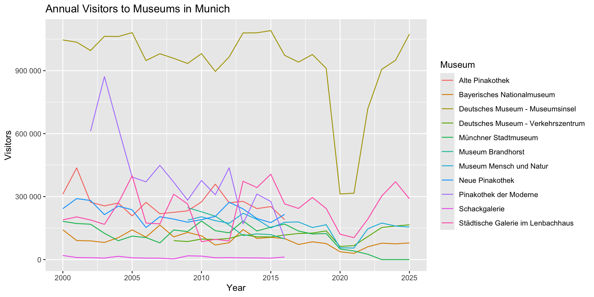
Example: Initial plots
Let’s plot museum_visitors as a line chart with monat on the x-axis, and wert on the y:
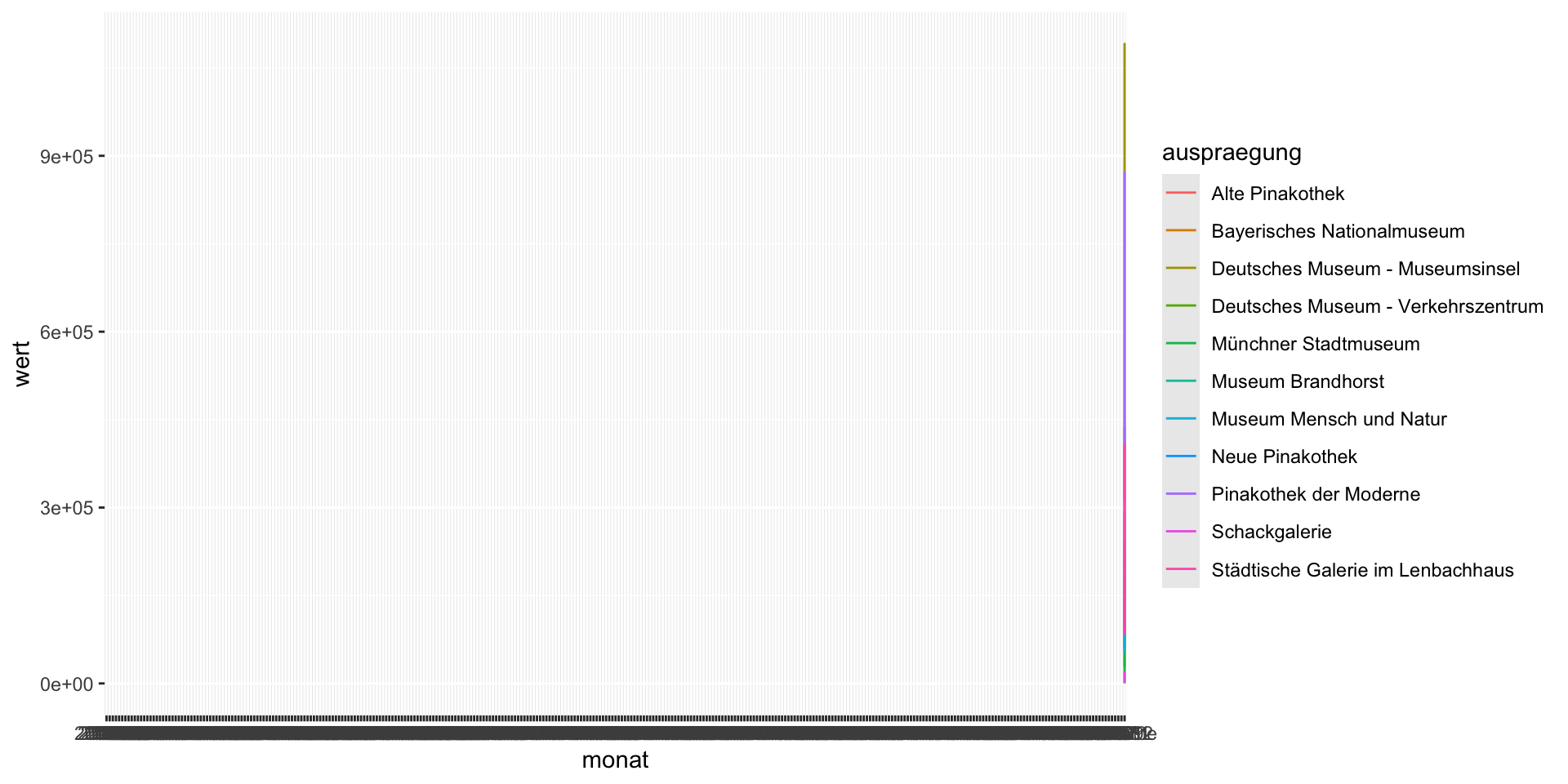
What went wrong?
- Why do you think there is a vertical line?
- Can you see data for all the museums?
- What was I assuming about the values in
monatandwert? - What should we investigate first?
Example: Screening the data
What do you notice about the column types?
Rows: 3,429
Columns: 9
$ monatszahl                     <chr> "Besucher*innen", "Besucher*innen", "Be…
$ auspraegung                    <chr> "Alte Pinakothek", "Alte Pinakothek", "…
$ jahr                           <dbl> 2026, 2026, 2026, 2026, 2026, 2026, 202…
$ monat                          <chr> "202601", "202602", "202603", "202604",…
$ wert                           <dbl> NA, NA, NA, NA, NA, NA, NA, NA, NA, NA,…
$ vorjahreswert                  <dbl> NA, NA, NA, NA, NA, NA, NA, NA, NA, NA,…
$ veraend_vormonat_prozent       <dbl> NA, NA, NA, NA, NA, NA, NA, NA, NA, NA,…
$ veraend_vorjahresmonat_prozent <dbl> NA, NA, NA, NA, NA, NA, NA, NA, NA, NA,…
$ zwoelf_monate_mittelwert       <dbl> NA, NA, NA, NA, NA, NA, NA, NA, NA, NA,…
Could we fix this with {lubridate} parsing?
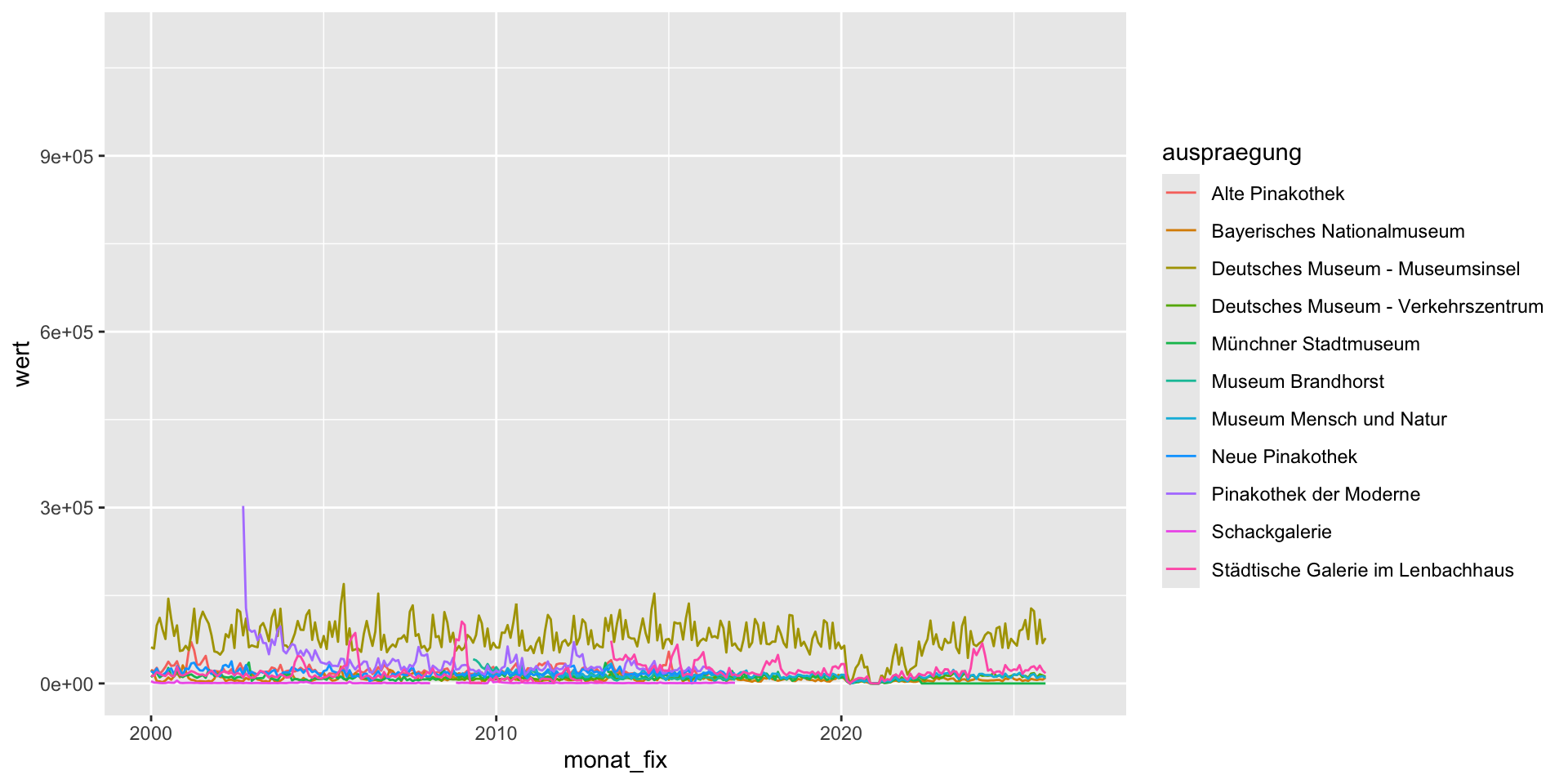
Example: Fixed data?
Did we correctly parse monat?
Rows: 3,429
Columns: 10
$ monatszahl                     <chr> "Besucher*innen", "Besucher*innen", "Be…
$ auspraegung                    <chr> "Alte Pinakothek", "Alte Pinakothek", "…
$ jahr                           <dbl> 2026, 2026, 2026, 2026, 2026, 2026, 202…
$ monat                          <chr> "202601", "202602", "202603", "202604",…
$ monat_fix                      <date> 2026-01-01, 2026-02-01, 2026-03-01, 20…
$ wert                           <dbl> NA, NA, NA, NA, NA, NA, NA, NA, NA, NA,…
$ vorjahreswert                  <dbl> NA, NA, NA, NA, NA, NA, NA, NA, NA, NA,…
$ veraend_vormonat_prozent       <dbl> NA, NA, NA, NA, NA, NA, NA, NA, NA, NA,…
$ veraend_vorjahresmonat_prozent <dbl> NA, NA, NA, NA, NA, NA, NA, NA, NA, NA,…
$ zwoelf_monate_mittelwert       <dbl> NA, NA, NA, NA, NA, NA, NA, NA, NA, NA,…
Example: Plot again!
No more data issues?
Example: Look again – overview
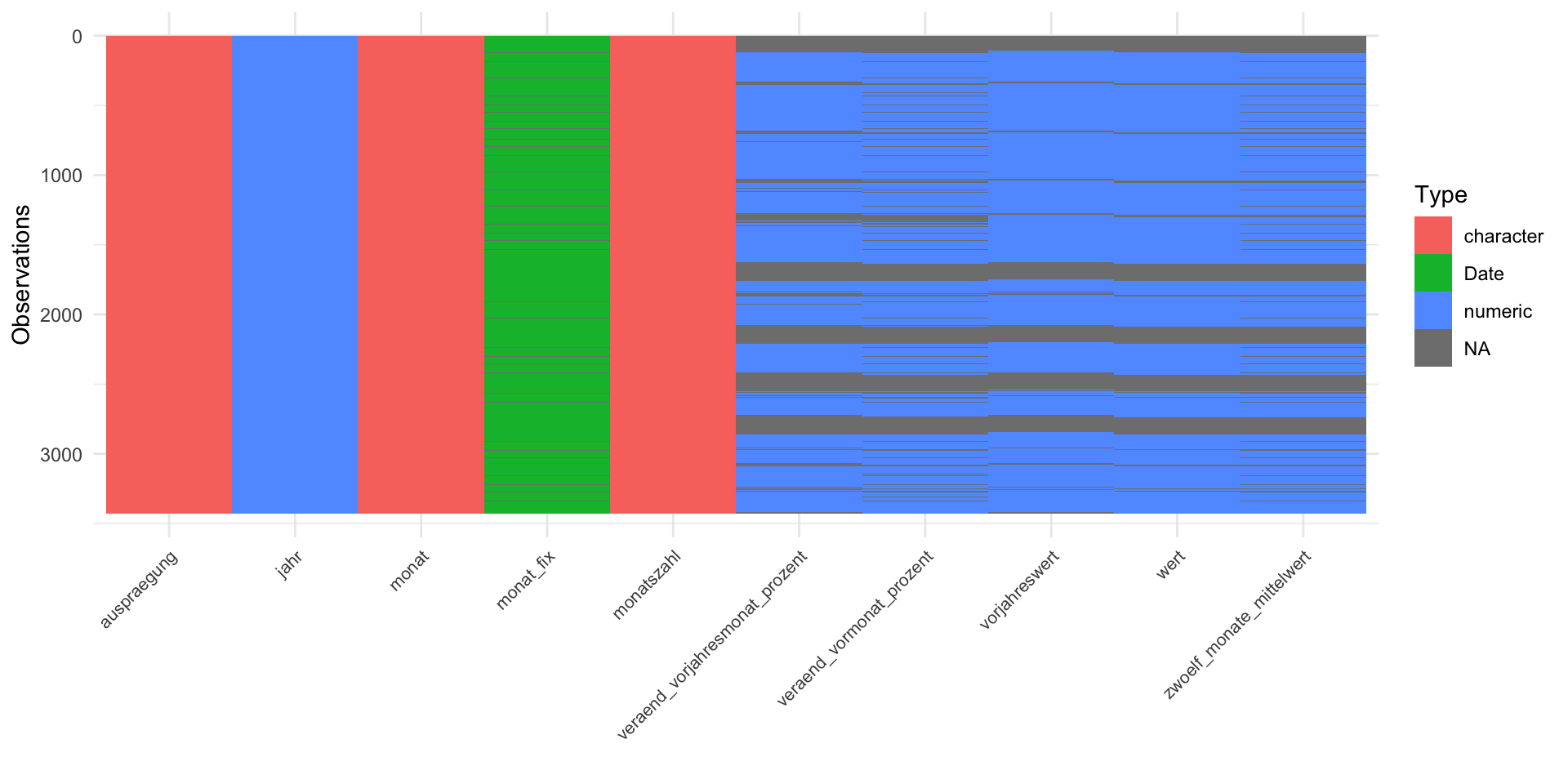
Example: Look again – closely
Do you notice anything odd in monat?
  [1] "202601" "202602" "202603" "202604" "202605" "202606" "202607" "202608"
  [9] "202609" "202610" "202611" "202612" "202501" "202502" "202503" "202504"
 [17] "202505" "202506" "202507" "202508" "202509" "202510" "202511" "202512"
 [25] "202401" "202402" "202403" "202404" "202405" "202406" "202407" "202408"
 [33] "202409" "202410" "202411" "202412" "202301" "202302" "202303" "202304"
 [41] "202305" "202306" "202307" "202308" "202309" "202310" "202311" "202312"
 [49] "202201" "202202" "202203" "202204" "202205" "202206" "202207" "202208"
 [57] "202209" "202210" "202211" "202212" "202101" "202102" "202103" "202104"
 [65] "202105" "202106" "202107" "202108" "202109" "202110" "202111" "202112"
 [73] "202001" "202002" "202003" "202004" "202005" "202006" "202007" "202008"
 [81] "202009" "202010" "202011" "202012" "201901" "201902" "201903" "201904"
 [89] "201905" "201906" "201907" "201908" "201909" "201910" "201911" "201912"
 [97] "201801" "201802" "201803" "201804" "201805" "201806" "201807" "201808"
[105] "201809" "201810" "201811" "201812" "201701" "201702" "201703" "201704"
[113] "201705" "201706" "201707" "201708" "201709" "201710" "201711" "201712"
[121] "Summe"  "201601" "201602" "201603" "201604" "201605" "201606" "201607"
[129] "201608" "201609" "201610" "201611" "201612" "201501" "201502" "201503"
[137] "201504" "201505" "201506" "201507" "201508" "201509" "201510" "201511"
[145] "201512" "201401" "201402" "201403" "201404" "201405" "201406" "201407"
[153] "201408" "201409" "201410" "201411" "201412" "201301" "201302" "201303"
[161] "201304" "201305" "201306" "201307" "201308" "201309" "201310" "201311"
[169] "201312" "201201" "201202" "201203" "201204" "201205" "201206" "201207"
[177] "201208" "201209" "201210" "201211" "201212" "201101" "201102" "201103"
[185] "201104" "201105" "201106" "201107" "201108" "201109" "201110" "201111"
[193] "201112" "201001" "201002" "201003" "201004" "201005" "201006" "201007"
[201] "201008" "201009" "201010" "201011" "201012" "200901" "200902" "200903"
[209] "200904" "200905" "200906" "200907" "200908" "200909" "200910" "200911"
[217] "200912" "200801" "200802" "200803" "200804" "200805" "200806" "200807"
[225] "200808" "200809" "200810" "200811" "200812" "200701" "200702" "200703"
[233] "200704" "200705" "200706" "200707" "200708" "200709" "200710" "200711"
[241] "200712" "200601" "200602" "200603" "200604" "200605" "200606" "200607"
[249] "200608" "200609" "200610" "200611" "200612" "200501" "200502" "200503"
[257] "200504" "200505" "200506" "200507" "200508" "200509" "200510" "200511"
[265] "200512" "200401" "200402" "200403" "200404" "200405" "200406" "200407"
[273] "200408" "200409" "200410" "200411" "200412" "200301" "200302" "200303"
[281] "200304" "200305" "200306" "200307" "200308" "200309" "200310" "200311"
[289] "200312" "200201" "200202" "200203" "200204" "200205" "200206" "200207"
[297] "200208" "200209" "200210" "200211" "200212" "200101" "200102" "200103"
[305] "200104" "200105" "200106" "200107" "200108" "200109" "200110" "200111"
[313] "200112" "200001" "200002" "200003" "200004" "200005" "200006" "200007"
[321] "200008" "200009" "200010" "200011" "200012"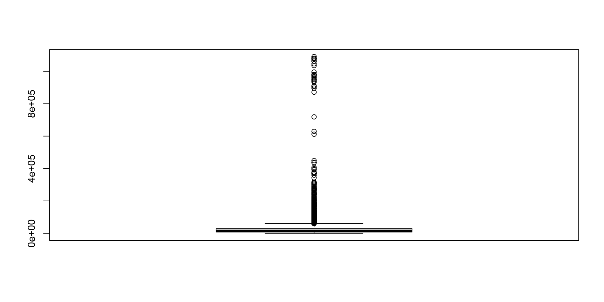
Example: ‘hidden’ annual data!
Notice that monat also contains the value Summe
# A tibble: 213 × 10
   monatszahl     auspraegung      jahr monat   wert vorjahreswert
   <chr>          <chr>           <dbl> <chr>  <dbl>         <dbl>
 1 Besucher*innen Alte Pinakothek  2016 Summe 189996        252404
 2 Besucher*innen Alte Pinakothek  2015 Summe 252404        242740
 3 Besucher*innen Alte Pinakothek  2014 Summe 242740        277484
 4 Besucher*innen Alte Pinakothek  2013 Summe 277484        270534
 5 Besucher*innen Alte Pinakothek  2012 Summe 270534        359183
 6 Besucher*innen Alte Pinakothek  2011 Summe 359183        274524
 7 Besucher*innen Alte Pinakothek  2010 Summe 274524        232143
 8 Besucher*innen Alte Pinakothek  2009 Summe 232143        225231
 9 Besucher*innen Alte Pinakothek  2008 Summe 225231        218386
10 Besucher*innen Alte Pinakothek  2007 Summe 218386        272646
# ℹ 203 more rows
# ℹ 4 more variables: veraend_vormonat_prozent <dbl>,
#   veraend_vorjahresmonat_prozent <dbl>, zwoelf_monate_mittelwert <dbl>,
#   monat_fix <date>
Example: Annual and Monthly rows?
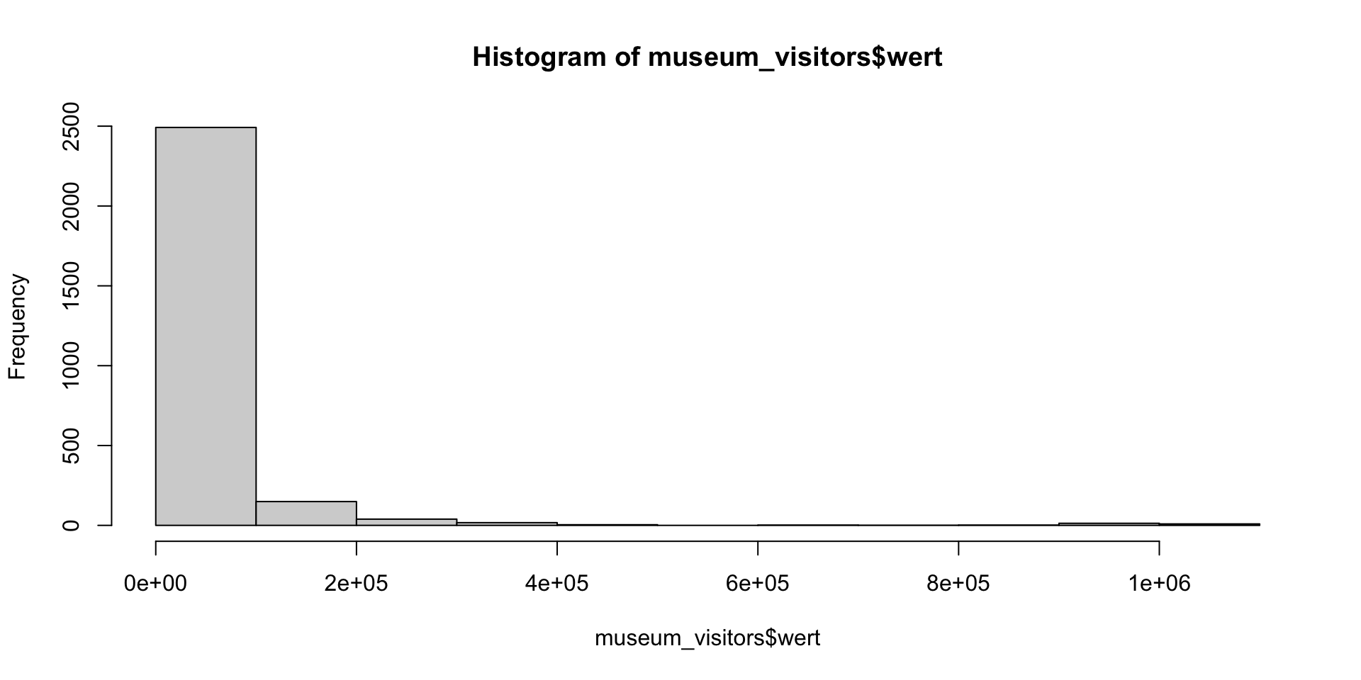
- What issues might arise if we didn’t know about the annual rows?
- How does this change your interpretation of the boxplot outliers?
Summary
IDA: Key ideas
- IDA is a systematic pre-analysis step — it checks data integrity without touching the research questions
- IDA issues occur at univariate, multivariate, and dataset levels — check all three
- Tidying (reshape/rename) ≠ cleaning (fix values/types) ≠ screening (characterise) — they overlap but have different goals
- All preparation decisions must be documented and justified in a reproducible script
Screening: Data types & formats
- Declare column types explicitly on import — avoid relying on guessing
- Use
lubridatefor dates; other specialist packages for geospatial (sf), time-of-day (hms), factors (forcats) etc. - Check every column: does the R type match the real-world meaning of the variable?
- Use
glimpse()for the whole table;str()for a single column
Cleaning: tools & fixes
- Plot first — histograms, boxplots, and line plots reveal issues that
summary()hides - Hypothesise before fixing — ask why a value looks wrong before deciding how to handle it
- Variable-level: recode types (
as.*()), flag/replace out-of-range values, standardise encodings - Structural: remove duplicates (
distinct()), reshape (pivot_*()), split/merge columns (separate(),unite()) - Not handling missingness is itself a decision — document it either way
Missingness
- Explicit missingness (
NA) — visible; find withis.na(),summary(),naniar::vis_miss() - Implicit missingness — absent rows; requires domain knowledge about expected structure
- Use
tidyr::complete()ortsibble::fill_gaps()to make implicit missingness explicit - The missing data mechanism (MCAR / MAR / MNAR) determines whether dropping or imputing is valid
For your group project
- Structure your data folder:
raw/(read-only) →interim/(.rdssnapshots) →final/ - Start every dataset with
glimpse(),summary(), and a plot — before writing any analysis code - Use
tidyr::complete()to surface implicit missingness in time-series data - Document why you made each data decision, not just what you did
- IDA findings may require revising your CDA plan — that is expected and normal
IDA in the oral exam
Aim to understand and explain:
- where your data comes from,
- what it tried to measure, what it actually measures
- if your questions and data match
- screening, tidying and cleaning issues and fixes
- missing data handling decisions
References
Chatfield, C. 1985. “The Initial Examination of Data.” Journal of the Royal Statistical Society. Series A (General) 148 (3): 214. https://doi.org/10.2307/2981969.
Huebner, Marianne, Saskia Le Cessie, Carsten Oliver Schmidt, and Lara Lusa. 2020. “Hidden Analyses: A Review of Reporting Practice and Recommendations for More Transparent Reporting of Initial Data Analyses.” BMC Medical Research Methodology 20 (1): 61. https://doi.org/10.1186/s12874-020-00942-y.
Huebner, Marianne, Saskia Le Cessie, Carsten O. Schmidt, and Werner Vach. 2018. “A Contemporary Conceptual Framework for Initial Data Analysis.” Observational Studies 4 (1): 171–92. https://doi.org/10.1353/obs.2018.0014.