Advanced Statistical Programming using R

Week 10: Analysis & Inference

2026-06-18

Announcements

This week

Project reminders
Oral exam preview
Learning from data
Planning for inference
{infer} package: tidy hypothesis testing

Upcoming deadlines

Progress Update due Jun 29
- Submit links to rendered website, project plan, and GitHub repo via Moodle
- We will provide group-specific feedback via GitHub issues

Group Project

Key dates

Milestone	Date	Submission
~~Draft Proposal~~	~~Jun 8~~	✓ general feedback in class today
Progress Update	29 Jun	URL to rendered site, updated Project Proposal
Group reflection — in-class discussion	W14 practical	N/A
Final submission + `group-reflection.qmd`	Due 22 Jul	URL to final website/webpage, group reflection doc
Individual contribution statement	Due 23 Jul	PDF via Moodle
Oral exam	29 Jul	—

From Proposals to Project Plans

Submitted proposals are Draft Project Plans:
- datasets & IDA: what data are you exploring?
- research questions: what are you trying to investigate or learn?
- analysis methods: how will you investigate your questions?
- data preparation: what preparation is required to interpret your data and conduct your planned analyses?
- final outputs: what formats will you use to document and present your analysis process and findings?
Continue to refine and update your project plans based on:
- applying concepts in Part 2: Working with Real World Data (W7-11)
- practising Part 1: Statistical Programming Skills (W2-6)

Project template

If you have not already set up your repo: use the template at https://github.com/soda-lmu/our-statprog2-project
Click Use this template on GitHub — it gives you the Quarto website structure and placeholder files to build on
If you already have a working repo: add a _quarto.yml to configure it as a website, make sure it renders, and use the template as a reference for what that looks like

Project final format

Adjust the navbar as needed for your output:

website:
  title: "StatProg2 Group Project"
  navbar:
    left:
      - href: index.qmd
        text: Home
      - href: proposal.qmd
        text: Proposal
      - href: report.qmd
        text: Report
      - href: Dashboard
        text: dashboard.qmd

Writing specific analysis plans

A specific plan names:

the response variable and each predictor
the method and why it fits your data structure
the null hypothesis — what would “no effect” look like?
what a meaningful result would look like

Vague:

“We will use regression to analyse the data.”

Specific:

“We will estimate bill_length_mm ~ body_mass_g + species using linear regression to test whether body mass predicts bill length after accounting for species differences.”

Null or boring results are fine!

Articulating why you did something matters more than getting every logical step perfectly correct
Focus on documenting your statistical decisions — handling missing data, sampling, etc.
We will not examine you on specific statistical techniques or methods, but statistical reasoning must be present for good statistical programming!

Oral Exam Preview

What the oral exam is looking for

Questions test reasoning and justification, not memorisation — we want to hear you think
Applying statistical concepts in code: what did you learn about using statistical ideas to draw conclusions from real data?
- data preparation and quality decisions
- modelling and method choices
- hidden assumptions or caveats in your findings
Communication choices: why did you visualise it this way? why this format?
Programming practices: code style, repo organisation, collaborative workflows
Tools you used and learnt: which packages, functions, or workflows did you choose — and why those over alternatives?

Sample questions

Part 2 — Applied statistics

“Did your dataset have any missingness? How did you handle it?”
“How did you choose this model, and how does it relate to your research question?”
“How did you interpret your results?”
“What reproducibility practices and tools did you use in your project and how?”
“Did you use LLMs in your project? For what tasks did it work well or not so well?”

Part 1 — Programming skills

“How would you decompose this code block into functions?”
“Describe a bug you investigated using debug() or browser().”
“What is one merge conflict you resolved?”
“From your project, what type of R package could you create?”

If you didn’t submit a project

We will show you an example dataset or output and ask equivalent questions:

“Here is a dataset — what cleaning steps would you take, and why?”
“Here is a test output — what was tested? What are the assumptions? Interpret the result.”
“Here is a variable codebook with gaps — what would you look for before starting analysis?”

Preparation advice

Practice explaining decisions and implementation out loud — to a classmate, a rubber duck, or yourself. For each step in your project, ask: why did I do it this way, how did I implement it, and what would I have done differently?

Last Week

Syllabus

Part 1: Statistical Programming Foundations

W02: Scripts, Functions & Refactoring
W03: Debugging
W04: Version Control & Remotes
W05: Quarto Websites & Collaborative Coding
W06: R Packages

Part 2: Working with Real World Data

W07: Initial Data Analysis & Data Cleaning
W09: Reproducibility, Open Data & renv
W10: Analysis & Inference
W11: Statistical Communication & Visualisation

Part 3: Advanced Topics & Summary

W12: Interactive Data Storytelling
W13: Multi-lingual Analysis (Python/R)
W14: Review & Outro

Reproducibility

Computational reproducibility: same data + same code → same results
renv fixes package versions; Docker fixes the full environment; Quarto + Git handle code and narrative
Reproducibility is a means — the goal is trustworthy, reusable, cumulative knowledge

renv

renv::init() creates a project-local library and records versions in renv.lock
renv::snapshot() updates the lockfile; renv::restore() rebuilds the library from it
Commit renv.lock to git; add renv/library/ to .gitignore

Open Data

Legal openness: know how to read and apply licences (CC0, CC BY, ODbL)
Technical openness: use standard, open formats (CSV, plain text)
FAIR: data should be Findable, Accessible, Interoperable, Reusable
Always document the licence, provenance, and context of any dataset you use

Documenting data analyses

Document decisions, not just actions — why at every stage (IDA, EDA, CDA)
Keep a reproducible script from raw data to clean data in data-raw/
State hypotheses before testing; disclose any deviations from plan
Well-organised data: consistent names, YYYY-MM-DD dates, one value per cell, plain text files

Learning from Data

Statistical inference across analysis goals

The fundamental problem

We observe a sample; we want to know about a population
The data we have is never the full picture
The key question: what can we legitimately say beyond the rows in our dataset?
Inference is how we make that leap — with a measure of uncertainty attached

%%{init: {'theme': 'base'}}%%
flowchart LR
    P(["🌍 Population (unknown)"])
    S(["📋 Sample (observed)"])
    S -- "inference ± uncertainty" --> P
    P -. "sampling" .-> S

Three goals of analysis

Descriptive: what is the state of things in the population?
- “What is the average bill length of Adelie penguins?”
Explanatory: is there a real relationship, and how strong is it?
- “Do heavier penguins tend to have longer flippers?”
Predictive: how well can we predict for a new, unseen case?
- “Given species and body mass, what flipper length would we expect?”
The goal determines the right method — and the right way to read the output

Three goals: at a glance

	Descriptive	Explanatory	Predictive
Core question	What is the state of things?	Is there a real relationship?	How well can we predict?
Penguin example	Mean bill length per species	Does body mass predict flipper length?	Predict flipper length for a new penguin
Inference licenses	Population estimates with uncertainty	Association or effect claims	Generalisation to new cases

Inference plays a different role in each goal

Descriptive: Is the mean bill length we observed a reliable estimate of the true population mean?
Explanatory: Is the relationship between body mass and flipper length real, or could it be sampling noise?
Predictive: Does a model trained on these penguins generalise to new ones it has never seen?
The same tools can appear across all three — but they are answering different questions

REVIEW: Linear regression

A linear regression model estimates the average value of a numeric outcome \(y\) as a linear function of one or more predictors \(x_1, x_2, \ldots\):

\[\hat{y} = \beta_0 + \beta_1 x_1 + \beta_2 x_2 + \cdots\]

Each coefficient \(\beta_i\) is the estimated change in \(y\) per one-unit increase in \(x_i\), holding other predictors fixed
The model is fit by minimising the sum of squared residuals (OLS)
In R: lm(y ~ x1 + x2, data = df)
You have seen this in Stat 1 & 2 — here we focus on how the goal changes what you do with the output

Linear regression & inference

The same lm() call can address either goal — what changes is how you read the output:

Descriptive: What is the average relationship between body mass and flipper length in this sample?
- The fitted line summarises the observed pattern — no population claim required
- Claim: “in this sample, flipper length increases by 0.015 mm per gram of body mass”
Explanatory: Is body mass associated with flipper length in the population, after accounting for species?
- Read the coefficient, its CI, and the p-value
- Claim: “a 1 g increase in body mass is associated with a 0.015 mm longer flipper (95% CI: …)”
Predictive: Given species and body mass, what flipper length do we expect for a new penguin?
- Read the predicted value and its prediction interval
- Claim: “we expect 185 mm (±12 mm) for an Adelie penguin weighing 3 500 g”
The model is identical — the question you bring to it is not

Statistical inference across analysis goals

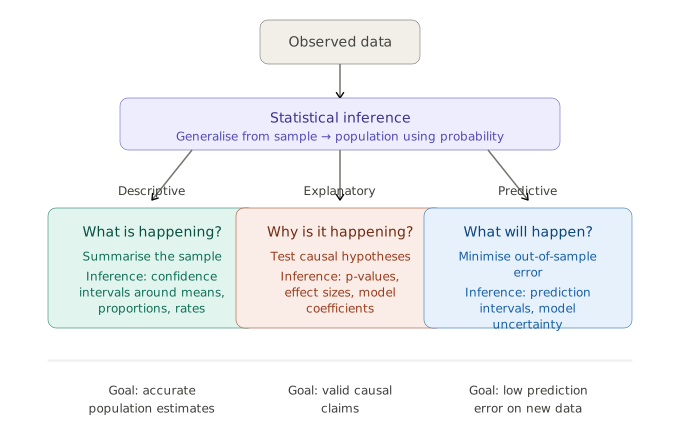
Inference tools by goal

	Descriptive	Explanatory	Predictive
Key question	Is this estimate reliable?	Is this real, and how large?	Does this generalise?
Point estimate	Mean, proportion, rate	Coefficient, effect size	Predicted value
Uncertainty	CI around the estimate	CI + hypothesis test	Prediction interval, cross-validation
Linear reg.	Summarise the sample relationship	Test whether coefficients are non-zero	Generate predictions for new cases
Common mistake	CI treated as a range of plausible individual values	p-value treated as proof of a causal relationship	Training accuracy reported as prediction accuracy

Exploratory vs confirmatory analysis

You will often hear “exploratory analysis” and “confirmatory analysis” used as labels — that is fine
But they are orthogonal to the analysis type: any descriptive, explanatory, or predictive analysis can be done exploratorily or confirmatorily
The distinction is about whether the question was fixed before or after looking at the data
Exploratory: the data suggests what to investigate — useful for generating hypotheses; treat any findings as provisional
- “I noticed Chinstrap penguins seem to have longer bills and then tested on fresh data”
Confirmatory: the question was fixed before looking — findings carry their full inferential guarantee
- “I pre-specified that bill depth would differ by species, then tested it”

Any analysis type can be exploratory or confirmatory

	Exploratory	Confirmatory
Descriptive	Plot all variables; report whichever summaries look interesting	Report pre-specified summaries (e.g. mean bill length per species)
Explanatory	Scan all variable pairs for associations; flag the strongest	Test one pre-specified relationship on a held-out sample
Predictive	Try many model variants; pick the one with the best-looking accuracy	Report accuracy on data held out before any modelling decisions were made

The two axes are independent: what you are trying to learn (type) vs. whether the question was fixed before you looked (exploratory/confirmatory).

CAUTION: Confirming after exploring

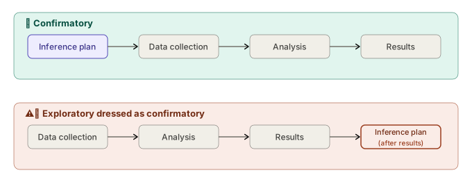
Planning for Inference

Two kinds of plan

A data analysis plan covers the full project: what data, what preparation, what methods, what outputs
An inference plan is focused on how you will learn from your data.
Describing, cleaning, and visualising data do not require an inference plan — the plan only matters when you make a claim that goes beyond the data you have.
Statistical software can make doing inference feel just like any other function, but the meaning and interpretation of inferential procedures does not come automatically when you output a p-value
Working with data in R is not the same as learning from data

Your data evidence budget

Every dataset arrives with a fixed amount of evidential currency — call it an evidentiary budget
Each time you look at the data to make a decision — which variables to examine, which patterns to follow up, which model to try — you spend some of that budget
When applying inferential tools (p-values, CIs, model metrics) you should account for how much has already been spent (e.g. via multiple testing adjustments)

Looking then testing

Running a test after noticing a pattern in your data is completely normal — and often the only option
What changes is what the p-value means: it was designed for a world where you asked one question, then collected data to answer it
When the data suggested the question, the p-value is still a valid number — but it is now describing a candidate finding, not a confirmed one
This is not about being careless — it is just what exploratory analysis is: using data to generate questions worth investigating further
Label findings honestly: “we noticed this pattern and ran a test” is a valid result; it just calls for replication, not headlines

Who wrote the question?

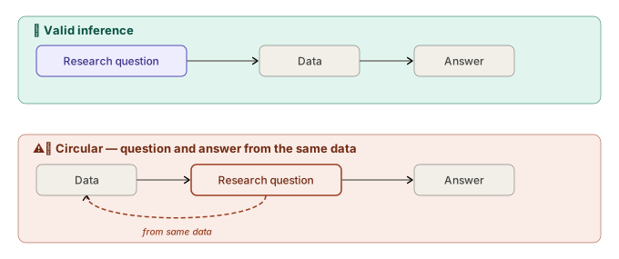
Example violations

Descriptive

Restaurant displaying only five-star reviews: If you calculate an average of 5-star reviews, the average (5) is calculated correctly, but the selection process means it cannot describe what customers actually think.

Explanatory

Reporting only the one significant result from twenty tests: If you run enough test variants, you’re bound to find some statistical artefact in the data, but the value of this evidence towards your original question is greatly (if not completely) reduced.

Predictive

Student who has seen the exam already: if you have already seen all the exam questions, your exam score tells you very little about how you would do on questions you have not seen. If you use all your data to train a model, and test it on the same data, it will be reproducing things it has already seen.

Keeping questions and answers separate

Pre-registration: write down your hypotheses and analysis plan before collecting (or touching) data
Sample splitting: set aside part of your data before exploring; run confirmatory tests only on the held-out portion
Cross-validation: rotate the hold-out across folds — useful when data is limited
Replication: test your finding on a new, independently collected dataset
The pattern from exploratory analysis becomes the pre-specified hypothesis for the next study

Navigating this in practice

Before you touch the data: write down — even informally — what you plan to examine and what you would need to see to draw a conclusion; a paragraph in a notebook or a comment at the top of a script is enough
While exploring: keep a record of what you tried — every subgroup checked, every variable considered and discarded, every model specification run
When reporting: distinguish clearly between what was pre-specified and what was discovered
- Pre-specified findings carry full inferential weight
- Exploratory findings are hypothesis-generating — real and worth reporting, but requiring fresh data before they become conclusions
Apply partial fixes: multiple comparisons corrections for descriptive work, sensitivity analyses for explanatory claims, strict hold-out evaluation for predictive models

This is genuinely hard

These mistakes appear constantly in published research, business analytics, and data journalism — including the replication crisis in psychology and medicine. They are not signs of incompetence. Knowing this should make you more careful, not less confident.

Real world prioritisation

Not every analysis needs the same level of inferential discipline. Ask two questions:

How consequential is the decision this analysis supports?
How much tolerance is there for being wrong?

Stakes	Tolerance for error	Investment in rigour
Dashboards, operational reports	Wide — decision support, not proof	Low
Business decisions, policy evaluation	Moderate	Medium
Clinical trials, legal evidence, systemic models	Narrow — getting it wrong is harmful	High

Statistics in a Court of Law?

🎙️ Law & Stats: What’s a Statistician Doing in Court? with Professor Ian Gordon, Episode 79, The Random Sample Podcast

The output of `lm()` is already inference

Every lm() summary contains hypothesis tests and confidence intervals — inference is built in
The t-test on each coefficient tests H₀: βᵢ = 0 — “is this predictor’s effect real, or sampling noise?”
The F-test tests H₀: all βᵢ = 0 — “does the model explain anything at all?”
These carry the same budget constraints as any other test: if the question came from the data, the p-values are optimistic
For your project: fitting a regression is doing inference — you still need to report it correctly and honestly

`{infer}`: Tidy Hypothesis Testing

From concepts to code

We have covered what inference is and when it is valid
This unit is about statistical programming — so let’s see what it actually looks like to implement this
We will focus on descriptive inference: estimating whether a pattern in our sample reflects a real difference in the population
Tool of choice: {infer} — a tidyverse-friendly package for hypothesis testing

Refresher: how hypothesis tests work

State the null hypothesis \(H_0\): assume there is no effect / no difference
Choose a test statistic that measures the size of the observed pattern (e.g. difference in means)
Build a null distribution: what values of the test statistic would you see if \(H_0\) were true?
Compare: how often does the null distribution produce a result as extreme as what you observed?
p-value: that frequency — small p means the observed result is unlikely under \(H_0\)

A p-value is not a probability that \(H_0\) is true

It is the probability of seeing a result at least this extreme, assuming \(H_0\) is true.

What should you test in your project?

Look at your descriptive summaries — which differences or patterns are worth asking “is this real?” about?
Match the test to your variable types:
- Two groups, continuous response → difference in means
- Two categorical variables → chi-square / difference in proportions
- Two continuous variables → correlation
When possible, state the null hypothesis in plain language before running the test — even one sentence is enough
If you are unsure which test fits, you can try using an LLM — describe your question and data — be sure to verify the suggestion (e.g. in the practical or via discussion board)
Your project analysis will mostly be exploratory, you can label findings as preliminary and note what fresh data would be needed to confirm them

Code setup

library(palmerpenguins)
library(dplyr)
library(infer)
library(tidyr)
library(ggplot2)

Start with description

penguins |> summary()

      species          island    bill_length_mm  bill_depth_mm  
 Adelie   :152   Biscoe   :168   Min.   :32.10   Min.   :13.10  
 Chinstrap: 68   Dream    :124   1st Qu.:39.23   1st Qu.:15.60  
 Gentoo   :124   Torgersen: 52   Median :44.45   Median :17.30  
                                 Mean   :43.92   Mean   :17.15  
                                 3rd Qu.:48.50   3rd Qu.:18.70  
                                 Max.   :59.60   Max.   :21.50  
                                 NA's   :2       NA's   :2      
 flipper_length_mm  body_mass_g       sex           year     
 Min.   :172.0     Min.   :2700   female:165   Min.   :2007  
 1st Qu.:190.0     1st Qu.:3550   male  :168   1st Qu.:2007  
 Median :197.0     Median :4050   NA's  : 11   Median :2008  
 Mean   :200.9     Mean   :4202                Mean   :2008  
 3rd Qu.:213.0     3rd Qu.:4750                3rd Qu.:2009  
 Max.   :231.0     Max.   :6300                Max.   :2009  
 NA's   :2         NA's   :2

Start with description

pCol <- c('#057076', '#ff8301', '#bf5ccb')
names(pCol) <- c('Gentoo', 'Adelie', 'Chinstrap')
plot(penguins, col = pCol[penguins$species], pch = 19)

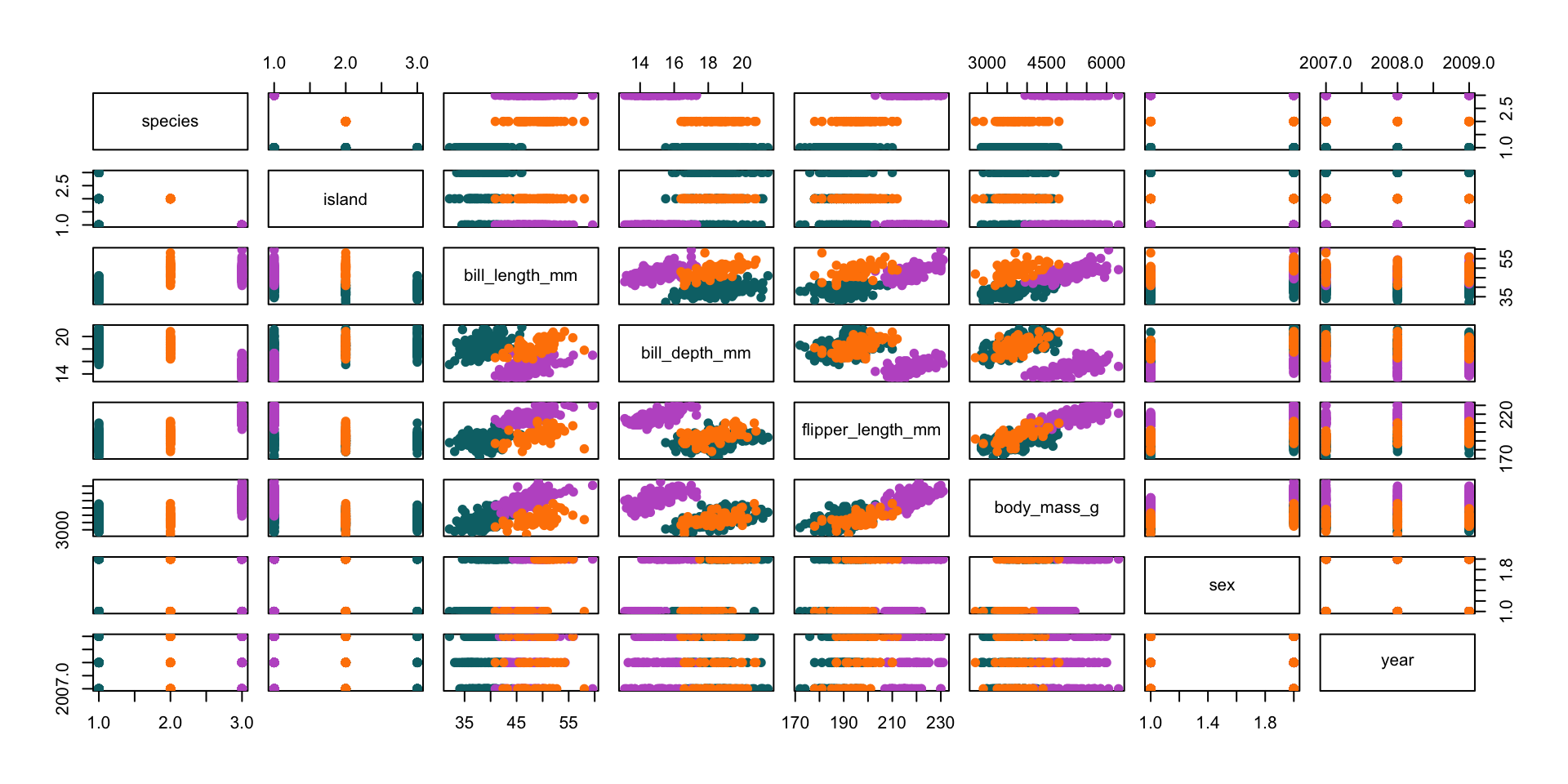
What is worth testing?

penguins |>
  group_by(species) |>
  summarise(
    n         = n(),
    mean_bill = mean(bill_length_mm, na.rm = TRUE),
    sd_bill   = sd(bill_length_mm, na.rm = TRUE)
  )

# A tibble: 3 × 4
  species       n mean_bill sd_bill
  <fct>     <int>     <dbl>   <dbl>
1 Adelie      152      38.8    2.66
2 Chinstrap    68      48.8    3.34
3 Gentoo      124      47.5    3.08

The summary suggests Adelie penguins have noticeably shorter bills than the other two species
But is that difference real in the population, or just sampling variation?
A descriptive question: “Is the mean bill length for Adelie penguins different from Chinstrap and Gentoo penguins in the population these birds were sampled from?”

Preparing to test

penguins_adelie <- penguins |>
  select(species, bill_length_mm) |>
  drop_na() |>
  mutate(adelie = if_else(species == "Adelie", "Adelie", "Non-Adelie"))

penguins_adelie |>
  group_by(adelie) |>
  summarise(
    n    = n(),
    mean = mean(bill_length_mm),
    sd   = sd(bill_length_mm)
  )

# A tibble: 2 × 4
  adelie         n  mean    sd
  <chr>      <int> <dbl> <dbl>
1 Adelie       151  38.8  2.66
2 Non-Adelie   191  48.0  3.23

The `{infer}` workflow

specify() — declare response and explanatory variables
assume(distribution) — use a theoretical null distribution ("t", "z", "Chisq", "F")
calculate(stat) — compute the observed test statistic from the data (must match the distribution)
get_p_value() — compute the p-value
get_confidence_interval(point_estimate) — compute a CI around the observed statistic
visualize() — plot the null distribution with the observed statistic and/or CI overlaid

Worked example: Adelie vs Chinstrap bill length

null_dist <- penguins_adelie |>
  specify(bill_length_mm ~ adelie) |>
  assume("t")

obs_stat <- penguins_adelie |>
  specify(bill_length_mm ~ adelie) |>
  calculate(stat = "diff in means", order = c("Adelie", "Non-Adelie"))

null_dist

A T distribution with 339 degrees of freedom.

obs_stat

Response: bill_length_mm (numeric)
Explanatory: adelie (factor)
# A tibble: 1 × 1
   stat
  <dbl>
1 -9.19

Visualise p-value

null_dist |>
  get_p_value(obs_stat = obs_stat, direction = "two-sided")

# A tibble: 1 × 1
   p_value
     <dbl>
1 4.12e-18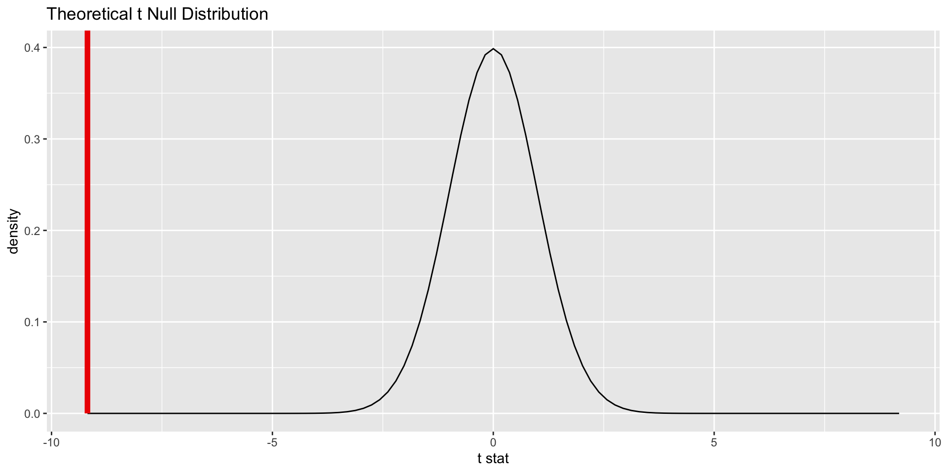

null_dist |>
  visualize() +
  shade_p_value(obs_stat = obs_stat, direction = "two-sided")

Calculate CI

ci <- null_dist |>
  get_confidence_interval(
    point_estimate = obs_stat,
    level          = 0.95
  )
ci

# A tibble: 1 × 2
  lower_ci upper_ci
     <dbl>    <dbl>
1    -9.81    -8.56

Interpretation

What the test gives evidence for

A large, precisely estimated difference in mean bill length: Adelie bills are ~8.78mm shorter than non-Adelie
95% CI entirely excludes zero: (−9.37, −8.19mm)
The difference is not plausibly attributable to sampling variation

What it does not establish

Why the difference exists (ecological adaptation, diet, foraging)
Whether island is a confounding variable — species and island are correlated in this dataset
Whether the non-Adelie group is homogeneous — it is not; Chinstrap and Gentoo differ from each other

Beware collapsing groups!

What could happen if Chinstrap and Gentoo mean bill lengths were either side of Adelie?
A one-way ANOVA across all three species, or pairwise t-tests with Bonferroni correction, would be more informative than the binary split used here

EXTENSION: simulation-based testing with `generate()`

assume("t") works because mathematicians derived what the null distribution looks like for common statistics — the t-distribution, chi-square, F, etc.
But what if your statistic does not have a known theoretical distribution? (e.g. a ratio, a trimmed mean, a custom score)
The alternative: simulate what the null world would look like by repeatedly shuffling the data and computing the statistic each time
After many shuffles, the distribution of those statistics is the null distribution — no formula required
This is called a permutation test (shuffling group labels) or bootstrap (resampling rows)

Note

For most standard tests (t, chi-square, ANOVA), assume() and generate() give essentially the same answer. generate() is most useful when you need a test that does not have a standard distribution.

EXTENSION: `generate()` in code

null_dist_sim <- penguins_adelie |>
  specify(bill_length_mm ~ adelie) |>
  hypothesize(null = "independence") |>
  generate(reps = 1000, type = "permute") |>
  calculate(stat = "diff in means", order = c("Adelie", "Non-Adelie"))

null_dist_sim |>
  visualize() +
  shade_p_value(obs_stat = obs_stat, direction = "two-sided") +
  labs(
    title = "Permutation null distribution — difference in mean bill length",
    subtitle = "Observed statistic shown in red",
    x = "Difference in means (mm)",
    y = "Count"
  )

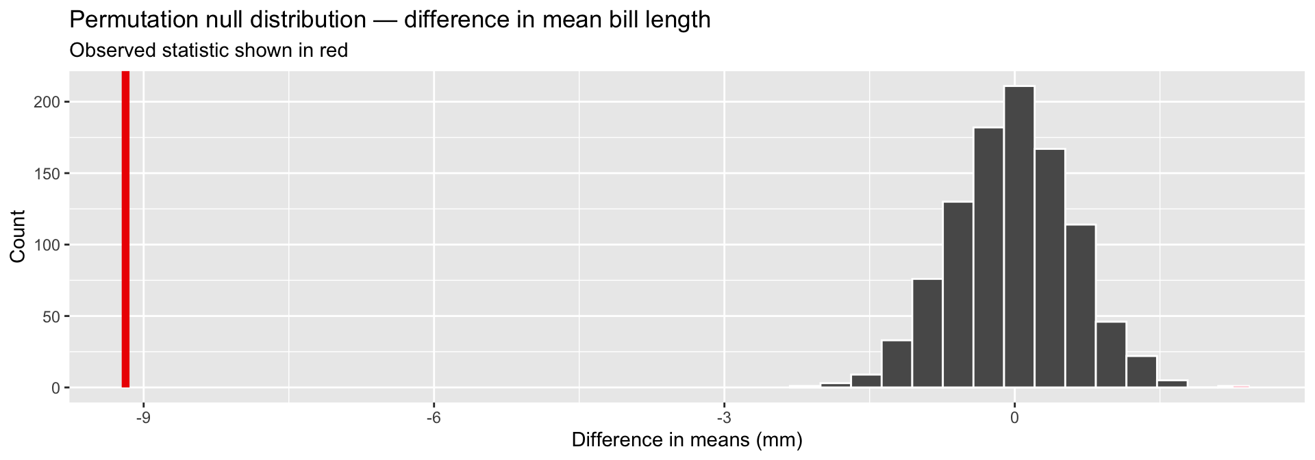
hypothesize(null = "independence") — states that species label and bill length are unrelated under \(H_0\)
generate(type = "permute", reps = 1000) — shuffles species labels 1000 times; each shuffle is one possible null world
calculate(stat = ...) — computes the statistic for every shuffle, building up the null distribution

Great explainer: Andrew Heiss, Null Worlds — https://nullworlds.andrewheiss.com

Why `{infer}`?

You already know t.test() and chisq.test() from Stat 1 & 2 — so why learn another tool?

The pipeline shape is the same whether you use theoretical distributions or simulation-based tests (assume() or generate()).
The package offers some statistical warnings and errors:

penguins |>
      specify(bill_length_mm ~ species) |>
      assume("t")

Error in `assume()`:
! The supplied distribution "t" is not well-defined for a numeric
  response variable (bill_length_mm) and a multinomial categorical explanatory
  variable (species).

Use what you already know

{infer} is one way to run inference in R — it is not the only way
The inferential techniques you covered in Stat 1, Stat 2, and StatProg 1 are all still valid: lm(), t.test(), chisq.test(), cor.test(), aov(), …
Hypothesis tests appear inside regression too — the t-tests on coefficients and the F-test for model fit are inference, not just model output
You are free to use base R, {infer}, or any other package that fits your analysis — what matters is that you can explain what test you are running and why

{broom} makes model output tidy

tidy(), glance(), and augment() from the {broom} package (part of the tidymodels ecosystem) convert lm(), glm(), and other model objects into data frames — easier to work with downstream than base R’s summary() output.

Summary

Learning from data

Three goals: descriptive (what is the state of things?), explanatory (is there a real relationship?), predictive (does this generalise?)
Exploratory vs confirmatory is orthogonal to the goal — any analysis type can be either; the distinction is whether the question was fixed before looking
Inference tools differ by goal: CIs for descriptive, hypothesis tests + effect sizes for explanatory, held-out evaluation for predictive

Planning for inference

A data analysis plan covers the full project; an inference plan is the component where you generalise beyond your sample
Running tests after exploring is normal — label those findings as exploratory/candidate and treat them as hypotheses for future work
Each look at the data spends some of the evidentiary budget — standard tools don’t adjust for this automatically
Write it down: even a paragraph before you start is enough to separate what you planned from what you discovered

`{infer}`

Workflow: specify() → assume() → calculate() → visualize() / get_p_value()
assume("t" / "z" / "Chisq" / "F") uses the same theoretical distributions as Stat 1/2
The null plot shows you where your test statistic sits in the null distribution
Extension: generate() simulates the null without assuming a distribution

Project tip: Updating your analysis plan

Know which type of analysis your project uses — descriptive, explanatory, predictive, or exploratory
EDA generates hypotheses; CDA tests them — keep the two steps distinct
A specific analysis plan should include your inferential strategy — the response, predictors, method, and null hypothesis

Project Tip: LLM-assisted planning

LLMs can help you: brainstorm methods, draft model specifications, find relevant packages
You must verify: variable names match your actual data, method assumptions hold, the test answers your question
Prompt for specifics: “Given response variable Y (continuous) and predictor X (categorical, 3 levels), what test should I use and why?”

Your responsibility

LLMs do not know your data. Check every suggestion against your actual dataset.

Teaching Evaluation

Your feedback matters (5 mins)

This is my first time teaching this course, and we rewrote the course pretty much from scratch
I would love to know what has worked well in the lectures and what could be improved.
Please only evaluate the lectures – there is a separate code for the practicals.

Please log on to:

https://www.lehrevaluation.uni-muenchen.de/evasys/public/online/index

Lösung: 4JQS5

Advanced Statistical Programming using R

Announcements

This week

Upcoming deadlines

Group Project

Key dates

From Proposals to Project Plans

Project template

Project final format

Writing specific analysis plans

Null or boring results are fine!

Oral Exam Preview

What the oral exam is looking for

Sample questions

If you didn’t submit a project

Last Week

Syllabus

Reproducibility

renv

Open Data

Documenting data analyses

Learning from Data

The fundamental problem

Three goals of analysis

Three goals: at a glance

Inference plays a different role in each goal

REVIEW: Linear regression

Linear regression & inference

Statistical inference across analysis goals

Inference tools by goal

Exploratory vs confirmatory analysis

Any analysis type can be exploratory or confirmatory

CAUTION: Confirming after exploring

Planning for Inference

Two kinds of plan

Your data evidence budget

Looking then testing

Who wrote the question?

Example violations

Keeping questions and answers separate

Navigating this in practice

Real world prioritisation

The output of lm() is already inference

{infer}: Tidy Hypothesis Testing

From concepts to code

Refresher: how hypothesis tests work

What should you test in your project?

Code setup

Start with description

Start with description

What is worth testing?

Preparing to test

The {infer} workflow

Worked example: Adelie vs Chinstrap bill length

Visualise p-value

Calculate CI

Interpretation

EXTENSION: simulation-based testing with generate()

EXTENSION: generate() in code

Why {infer}?

Use what you already know

Summary

Learning from data

Planning for inference

{infer}

Project tip: Updating your analysis plan

Project Tip: LLM-assisted planning

Teaching Evaluation

Your feedback matters (5 mins)

The output of `lm()` is already inference

`{infer}`: Tidy Hypothesis Testing

The `{infer}` workflow

EXTENSION: simulation-based testing with `generate()`

EXTENSION: `generate()` in code

Why `{infer}`?

`{infer}`