Advanced Statistical Programming using R

Week 13: Multi-lingual Analysis (Python/R)

2026-07-09

Announcements

Repo review

• Feedback on your repo review will be posted on Moodle this week.

Oral exam

• Reach out to statprog@stat.uni-muenchen.de if you have any special requirements, e.g.:
  • time conflicts with other exams on the same day
  • language restrictions
• We are going to send you your time slots by next week.
• Location: Zoom

Retake exam

Upcoming deadlines

• Final submission due 22 Jul
  • URL to final website/webpage + group-reflection.qmd
• Individual contribution statement due 23 Jul (PDF via Moodle)
• Oral exam: 29 Jul

Syllabus

Part 1: Statistical Programming Foundations

• W02: Scripts, Functions & Refactoring
• W03: Debugging
• W04: Version Control & Remotes
• W05: Quarto Websites & Collaborative Coding
• W06: R Packages

Part 2: Working with Real World Data

• W07: Initial Data Analysis & Data Cleaning
• W09: Reproducibility, Open Data & renv
• W10: Analysis & Inference
• W11: Statistical Communication & Visualisation

Part 3: Advanced Topics & Summary

• W12: Interactive Data Storytelling
• W13: Multi-lingual Analysis (Python/R)
• W14: Review & Outro

Last Week

Interactive visualisation

• htmlwidgets (plotly, leaflet, DT) add interactivity to any Quarto HTML output — no server required
• ggplotly() is the quickest path from a ggplot2 plot to an interactive one
• Observable JS in Quarto enables reactive, filter-driven views without a Shiny server
• Shiny is the right tool when you need server-side computation or persistent state

Geospatial visualisation

• {sf} + geom_sf() for choropleth and boundary maps with proper projection handling
• {geofacet} for small-multiple comparisons arranged in a geographic layout
• Choose based on whether exact geography or spatial comparison of trends is the goal

Interactivity in one line

Any ggplot2 figure becomes explorable with ggplotly() — hover, zoom, toggle groups:

p <- ggplot(penguins, aes(bill_length_mm, body_mass_g, colour = species)) +
  geom_point(alpha = 0.7) +
  labs(x = "Bill length (mm)", y = "Body mass (g)", colour = "Species") +
  theme_minimal()

ggplotly(p)

• 1-minute recap demo: hover a point, click a legend entry to hide a species
• Bridge to today: this plot reappears later — drawn in Python

This Week

Multi-lingual analysis

• Problems and limitations of R
• A different perspective: Python
  • what it is, how it compares to R
  • fundamentals, side by side with R
• The best of both worlds: {reticulate}
  • Python inside R, R inside Python
  • when to use which language

This is not a Python course

Expectations for this session

You are not expected to become proficient in Python today. You should leave being able to

1. read and understand basic Python code,
2. explain what reticulate does and how it works,
3. reason about when to use R vs Python in a data science workflow.

• Manage expectations up front — one session cannot teach a language
• The comparison format is deliberate: they already know the R side, so the Python side is a translation exercise, not new material

Problems and Limitations of R

R is a domain-specific language

• R was designed by statisticians, for statistics — and it shows, in the best way:
  • vectorised operations, NA as a first-class citizen, formulas (y ~ x), data frames built in
  • unmatched ecosystem for statistical inference and visualisation
• But the same design brings limitations:
  • speed: interpreted loops are slow
  • memory: objects are copied more than you might expect
  • OOP: several competing class systems
  • ecosystem gaps: some fields live elsewhere

• Frame positively: limitations are the flip side of design decisions that make R great at statistics
• Each bullet gets its own slide with a code example next

Limitation 1: loops are slow

Summing a million numbers — a for loop versus the vectorised built-in:

x <- rnorm(1e6)

sum_loop <- function(x) {
  total <- 0
  for (xi in x) total <- total + xi
  total
}

system.time(for (i in 1:50) sum_loop(x))["elapsed"]

elapsed 
  0.522 

system.time(for (i in 1:50) sum(x))["elapsed"]

elapsed 
  0.046 

Tip

Vectorised R functions call fast compiled C code. The R interpreter is slow; the libraries are not. Python has exactly the same split: plain loops are slow, numpy is fast.

• ~2 orders of magnitude difference — let students guess the factor before revealing
• Key nuance: this is a property of interpreted languages, not R specifically — pure-Python loops are just as slow
• The escape hatches: vectorise, or drop to C++ (Rcpp) — or another language

Limitation 2: R copies your data

When you change part of an object, R makes a fresh copy rather than editing the original in place:

x <- c(1, 2, 3)
y <- x            # y looks like the same data as x...
y[1] <- 99        # ...but changing y

x                 # leaves x untouched — R copied it behind the scenes

[1] 1 2 3

Tip

This makes R safe and predictable: nothing changes unless you assign it. The cost: for a very large dataset, every small edit can duplicate it — slow and memory-hungry. pandas/numpy edit data in place instead, trading a little safety for speed.

• The teaching point is value semantics, kept abstract: “R copies rather than sharing” — no need for tracemem or memory addresses
• Ask: is x changed after we edited y? (No.) That safety is the upside
• Downside only bites at scale: editing one cell of a huge data frame can copy the whole thing
• The escape hatches (data.table, arrow) exist, but the point here is just the tradeoff vs Python

A detour: what is object-oriented programming?

So far we have written functions: data goes in, a result comes out. As programs grow, two wishes appear:

• bundle data together with the operations that belong to it
• have the same command do the right thing for different kinds of data

That is object-oriented programming (OOP):

• a class is a blueprint for a kind of thing (a data frame, a fitted model, a plot)
• a method is a function that belongs to that class and knows how to handle it

Tip

You have used this all semester without naming it: summary() prints group means for a data frame but coefficients and p-values for a model. One command, many behaviours — the object decides.

• Keep it gentle — most students have never met OOP formally
• Anchor on something familiar: summary()/print()/plot() already adapt to their input; that adaptation IS method dispatch
• Blueprint vs instance: “class = cookie cutter, object = cookie” is a useful one-liner
• This also sets up Python’s df.groupby().mean() method syntax later — methods attached to objects

Limitation 3: which OOP system?

Most languages give you one way to build classes and methods. R has several — and the oldest (S3) trusts you so completely you can lie about a class:

x <- 1:3
class(x) <- "lm"   # S3: a class is just an attribute...
summary(x)         # ...and dispatch happily takes our word for it

Error in z$rank: $ operator is invalid for atomic vectors

System	Style	Used by
S3	informal, convention-based	most of base R, dplyr, ggplot2
S4	formal classes + validation	Bioconductor, Matrix
R6	encapsulated, mutable	shiny, plumber
S7	successor unifying S3/S4	new packages (emerging)

• S3 dispatch trusts the class attribute blindly — the error comes from deep inside summary.lm, not from a type check
• Contrast with next section: Python has ONE class system, and class is a keyword
• Don’t teach S4/R6 details — the point is fragmentation, not mechanics

Limitation 4: ecosystem gaps

Some fields are simply Python-first — the reference implementations live there:

• Deep learning: PyTorch, TensorFlow, JAX (R wrappers exist — they call Python underneath)
• Modern ML tooling: scikit-learn’s uniform API, Hugging Face transformers
• Production & glue: web backends, cloud SDKs, task schedulers, robotics, …
• General-purpose programming: Python is a top choice far beyond data science

Note

The reverse holds too: mixed models, survey statistics, econometrics, and publication-grade graphics are R-first. That asymmetry is exactly why multi-lingual workflows exist.

• {keras3} and {torch} in R are wrappers/reimplementations — the community, docs, and cutting edge are in Python
• Ask students: which of these gaps matter for YOUR project? For most course projects: none — R is the right tool here

A Different Perspective: Python

What is Python?

• General-purpose, interpreted, dynamically typed language — created by Guido van Rossum, first released 1991 (R: 1993)
• Design goal: readability — indentation is the syntax
• Runs everywhere: scripting, web servers, ML pipelines, embedded systems
• Batteries via libraries: data science lives in numpy, pandas, matplotlib/seaborn, scikit-learn — not in the core language
• The most-used programming language in Stack Overflow’s developer survey; #1 on the TIOBE index

• Base Python ships without a data frame or a plot function — everything statistical is a library
• That’s the deep contrast: R’s core IS statistics; Python’s core is general programming
• Popularity matters practically: more tutorials, more Stack Overflow answers, more job ads

R vs Python at a glance

	R	Python
Designed for	statistics & data analysis	general-purpose programming
Data frame	built in	pandas library
Missing values	NA in the core language	NaN/None, library-dependent
Indexing	starts at 1	starts at 0
Assignment	x <- 1	x = 1
OOP	S3/S4/R6/S7	one class system
Typical style	functions + pipes: df |> f()	methods on objects: df.f()
Killer apps	inference, ggplot2, Quarto/Shiny	ML/DL, glue code, web

Tip

Both are interpreted, dynamically typed, open source, and slow in raw loops but fast through compiled libraries. The concepts you learned this semester transfer — only the syntax changes.

• Spend a minute here — this table is the mental map for the whole section
• Emphasise the last row of similarities: they already know 90% of what matters

Basics: assignment & arithmetic

The same computation, side by side — spot the differences:

R

x <- 10
y <- 3
x / y

[1] 3.333333

x == y   # equality

[1] FALSE

x || y    # or

[1] TRUE

x^y

[1] 1000

Python

x = 10
y = 3
x / y

3.3333333333333335

x == y    # equality

False

x or y     # or (wait, what?)

10

x**y

1000

• Reveal R first, let students guess the Python column before showing it
• Differences: = for assignment, // vs %/%, ** vs ^, # comments identical
• Meta-point in the callout: this deck itself is a multi-lingual document — foreshadow reticulate

Vectors vs lists — and 0-based indexing

How would Python write this? (guess before revealing)

R — the atomic vector

x <- c(10, 20, 30, 40)
x[1]        # first element

[1] 10

x[2:3]      # slice (inclusive)

[1] 20 30

x * 2       # vectorised!

[1] 20 40 60 80

Python — the list

x = [10, 20, 30, 40]
x[0]        # first element!

10

x[1:3]      # end is EXCLUSIVE

[20, 30]

x * 2       # ...repetition?!

[10, 20, 30, 40, 10, 20, 30, 40]

Important

Three classic traps: Python counts from 0, slices exclude the end, and lists are not vectorised — x * 2 repeats the list. Element-wise maths needs numpy: np.array(x) * 2.

• THE slide of the session — let students predict all three outputs, most will get x * 2 wrong
• x[1:3] returns elements 2 and 3 (indices 1, 2) — compare with R’s inclusive 2:3 giving the same values by different logic
• numpy arrays behave like R vectors: np.array([10,20,30,40]) * 2 — show in console if time

Containers Python has (and R sort of has)

Python first this time — what would you use in R for each of these?

R — collections

ages = list(anna = 31, ben = 25)      # named list
point = c(48.15, 11.58)               # numeric vector
species = unique(c("adelie", "gentoo", "adelie"))  # unique elements
paste(ages$anna, point[1], paste(species, collapse = ", "))

[1] "31 48.15 adelie, gentoo"

Python — collections

ages = {"anna": 31, "ben": 25}        # dictionary: key -> value
point = (48.15, 11.58)                # tuple: immutable
species = {"adelie", "gentoo", "adelie"}  # set: unique elements
print(ages["anna"], point[0], species)

31 48.15 {'gentoo', 'adelie'}

Python	Closest R equivalent
dict — {"a": 1}	named list / named vector: list(a = 1)
tuple — (1, 2)	no direct equivalent (immutable)
set — {1, 2}	unique(x) + union(), intersect()
list — [1, 2]	list(1, 2) (R lists hold anything too)

• Ask the room for each line before showing the table
• dict is everywhere in Python — JSON maps to dicts, function options are dicts
• The set silently dropped the duplicate “adelie” — point at the printed output
• Sets/dicts are hash-based: fast membership tests, no order guarantees (dicts keep insertion order since 3.7)

Functions

R

standardise <- function(x, center = TRUE) {
  if (center) x <- x - mean(x)
  x / sd(x)
}

standardise(c(2, 4, 6, 8))

[1] -1.1618950 -0.3872983  0.3872983  1.1618950

Python

import numpy as np

def standardise(x, center=True):
    if center:
        x = x - np.mean(x)
    return x / np.std(x, ddof=1)

standardise(np.array([2, 4, 6, 8]))

array([-1.161895  , -0.38729833,  0.38729833,  1.161895  ])

Important

No braces: the indented block is the function body — wrong indentation is a syntax error. And return is mandatory; Python functions don’t auto-return the last expression.

• def vs function, = for defaults in both — but no spaces around = in Python defaults by convention
• ddof=1: numpy’s std divides by n by default; ddof=1 gives the sample sd matching R — nice “trust but verify” example
• import numpy as np — libraries are imported under a namespace alias; like library() but you keep the prefix

Loops & conditionals

R

sizes <- c(1, 15, 200)
for (n in sizes) {
  if (n < 10) {
    print("small")
  } else if (n < 100) {
    print("medium")
  } else {
    print("large")
  }
}

[1] "small"
[1] "medium"
[1] "large"

Python

sizes = [1, 15, 200]
for n in sizes:
    if n < 10:
        print("small")
    elif n < 100:
        print("medium")
    else:
        print("large")

small
medium
large

Tip

Python’s list comprehension replaces many explicit loops — closer to R’s sapply()/purrr::map() than to a for loop:

[n**2 for n in sizes if n < 100]

[1, 225]

• Same logic, same keywords almost — elif vs else if, colon + indentation vs braces + parens
• No parentheses around the condition in Python
• Comprehensions are idiomatic Python — students WILL meet them when reading Python code; practical Ex 1.1 has one

dplyr vs pandas — wrangling

The penguins, filtered and summarised — same pipeline, two grammars:

R — functions piped over data

penguins |>
  filter(!is.na(body_mass_g)) |>
  group_by(species) |>
  summarise(
    n = n(),
    mass = mean(body_mass_g)
  )

# A tibble: 3 × 3
  species       n  mass
  <fct>     <int> <dbl>
1 Adelie      151 3701.
2 Chinstrap    68 3733.
3 Gentoo      123 5076.

Python — methods chained on the object

penguins = r.penguins   # (!) the R data frame

(penguins
  .dropna(subset=["body_mass_g"])
  .groupby("species", observed=True)
  .agg(n=("body_mass_g", "size"),
       mass=("body_mass_g", "mean"))
)

             n         mass
species                    
Adelie     151  3700.662252
Chinstrap   68  3733.088235
Gentoo     123  5076.016260

• r.penguins: Python reads the R object directly — reticulate at work, banner for the next section
• The chain of methods .dropna().groupby().agg() == the pipe chain; wrap in ( ) to split over lines
• observed=True: silences pandas’ categorical-groupby warning; don’t dwell
• Row order and results match — let students map each verb to its counterpart

dplyr vs pandas — verb dictionary

dplyr	pandas
filter(mass > 4000)	df[df["mass"] > 4000] or df.query("mass > 4000")
select(species, mass)	df[["species", "mass"]]
mutate(kg = mass / 1000)	df.assign(kg = df["mass"] / 1000)
arrange(desc(mass))	df.sort_values("mass", ascending=False)
group_by(g) |> summarise(m = mean(x))	df.groupby("g")["x"].mean()
left_join(df2, by = "id")	df.merge(df2, on="id", how="left")
rename(new = old)	df.rename(columns={"old": "new"})

Tip

Keep this table (and an LLM) at hand and you can read most pandas code today. The verbs are the same ideas — you learned the concepts in week 7, not just the syntax.

• Don’t read every row aloud — highlight filter (boolean mask idiom is the big syntactic difference) and join (merge)
• LLMs are excellent at dplyr↔︎pandas translation precisely because it’s mechanical — but you must be able to VERIFY the output (reflection prompt this week)

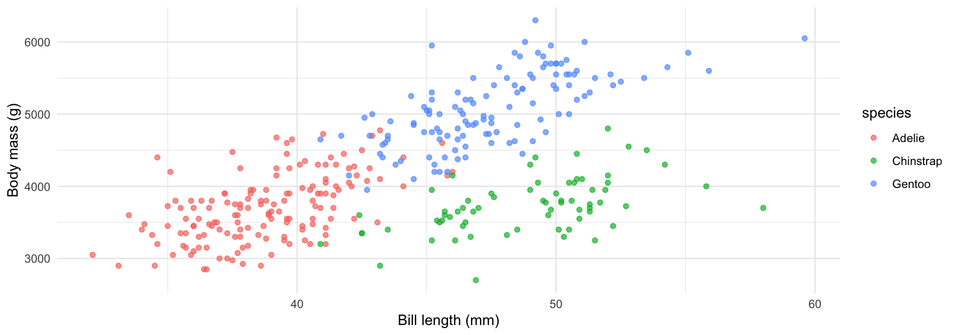
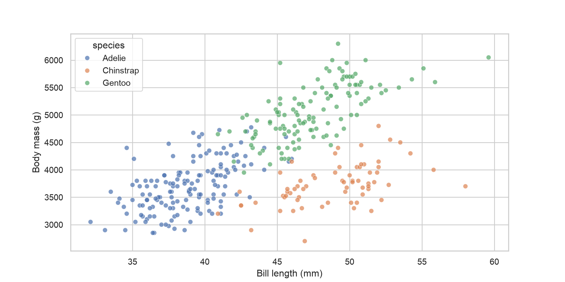
ggplot2 vs seaborn — scatter

R — grammar of graphics

ggplot(penguins,
       aes(bill_length_mm, body_mass_g,
           colour = species)) +
  geom_point(alpha = 0.7) +
  labs(x = "Bill length (mm)",
       y = "Body mass (g)") +
  theme_minimal()

Python — one function per chart type

import seaborn as sns
import matplotlib.pyplot as plt

sns.set_theme(style="whitegrid")
sns.scatterplot(penguins,
                x="bill_length_mm",
                y="body_mass_g",
                hue="species", alpha=0.7)
plt.xlabel("Bill length (mm)")
plt.ylabel("Body mass (g)")
plt.show()

• Same figure, both actually rendered — aes() ↔︎ x=/y=/hue=, alpha identical
• seaborn sits on matplotlib the way ggplot sits on grid — labels are set via plt on the current figure
• No layered grammar: seaborn has one function per chart type (scatterplot, histplot, boxplot…) instead of composable geoms
• hue = colour aesthetic; seaborn handles the legend automatically

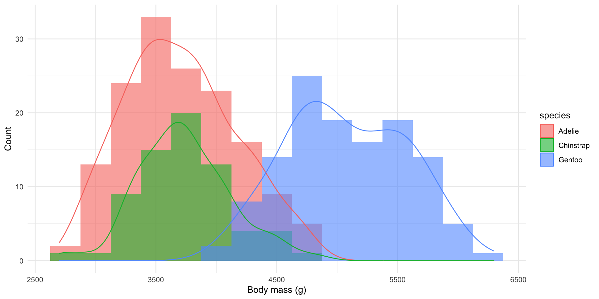
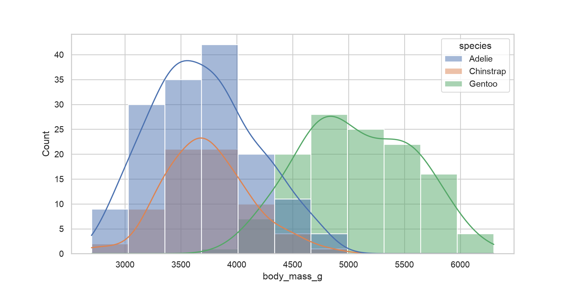
ggplot2 vs seaborn — distributions

Python first — what’s the ggplot2 equivalent? (guess, then reveal)

R

ggplot(penguins,
       aes(body_mass_g, fill = species)) +
  geom_histogram(binwidth = 250, alpha = 0.6,
                 position = "identity") +
  geom_density(aes(y = after_stat(count) * 250,
                   colour = species),
               fill = NA) +
  labs(x = "Body mass (g)", y = "Count") +
  theme_minimal()

Python

sns.histplot(penguins, x="body_mass_g",
             hue="species", kde=True)
plt.show()

• Reversed direction on purpose: read the Python, predict the R
• kde=True overlays a density — in ggplot that’s a second geom, and scaling density to count needs the after_stat trick (× binwidth)
• Honest take: THIS plot is less work in seaborn; the fully polished, publication-grade version is less work in ggplot2

Where Python shines: scikit-learn

Every model — regression, trees, boosting, SVMs — has the same fit/predict API:

from sklearn.model_selection import train_test_split
from sklearn.ensemble import RandomForestClassifier

df = penguins.dropna(subset=["bill_length_mm", "flipper_length_mm", "body_mass_g"])
X, y = df[["bill_length_mm", "flipper_length_mm", "body_mass_g"]], df["species"]
X_train, X_test, y_train, y_test = train_test_split(X, y, random_state=13)

model = RandomForestClassifier(n_estimators=100).fit(X_train, y_train)
round(model.score(X_test, y_test), 3)   # accuracy on held-out data

0.965

Also typically easier in Python: deep learning (PyTorch), NLP/LLMs (Hugging Face transformers), gluing APIs and services together. R’s counterpart {tidymodels} is excellent — but the ML ecosystem’s centre of gravity is Python.

• The point is the API design, not random forests: swap RandomForestClassifier for LogisticRegression and NOTHING else changes
• train/test split + held-out accuracy in 6 lines — this uniformity is why ML courses teach sklearn
• ~97–100% accuracy: penguin species are nearly separable from these three measurements
• Bridge to next section: “so we need Python for the model — do we abandon R? No.”

The Best of Both Worlds: reticulate

Based on: rstudio.github.io/reticulate

What is {reticulate}?

• An R package that runs an embedded Python session inside your R session
• Python and R objects are translated automatically in both directions
• You can:
  • run Python code and scripts from R (py_run_string(), source_python())
  • import any Python module as an R object (import("numpy"))
  • mix ```{r} and ```{python} chunks in one Quarto document — these slides do exactly that
• Named after the reticulated python 🐍 — the snake, not the language

• One process, one workspace spanning two languages — not “export CSV, run script, import CSV”
• Every Python output in the previous section was produced through reticulate
• Point at the setup chunk: library(reticulate); use_virtualenv(...) is ALL the configuration this deck needed

How objects cross the border

Conversion is automatic and (mostly) lossless:

R	→	Python
single value (1, "a", TRUE)	↔︎	scalar (1.0, "a", True)
vector c(1, 2, 3)	↔︎	list [1.0, 2.0, 3.0]
matrix / array	↔︎	numpy array
named list list(a = 1)	↔︎	dict {"a": 1.0}
data.frame	↔︎	pandas DataFrame
NULL	↔︎	None

Note

Two bridges, one workspace: in R, py$x reads Python’s x; in Python, r.x reads R’s x. That’s how r.penguins worked earlier.

• Watch out: R has no scalar type — a length-1 vector becomes a Python scalar, not a list; wrap in list() if a list is required
• 1-element gotchas aside, students rarely need to think about conversion — it just works
• The r./py$ symmetry is the key mental model for the practical

Calling a Python function from R

Define a function in a Python chunk…

def rescale(x, lo=0.0, hi=1.0):
    """Scale values in x linearly to the range [lo, hi]."""
    xmin, xmax = min(x), max(x)
    return [lo + (v - xmin) * (hi - lo) / (xmax - xmin) for v in x]

…then call it from R via py$, with plain R vectors as arguments:

measurements <- c(4.2, 5.0, 3.1, 6.4)
py$rescale(measurements, lo = 0, hi = 10)

[1]  3.333333  5.757576  0.000000 10.000000

Tip

For .py files instead of chunks: source_python("helpers.py") makes every function in the file directly callable from R — exactly what you’ll do in the practical.

• The R vector arrives as a Python list, the returned list comes back as an R vector — zero manual conversion
• Named arguments work across the border too (lo =, hi =)
• Practical Ex 1.2 is this pattern with a sum function — call it out explicitly

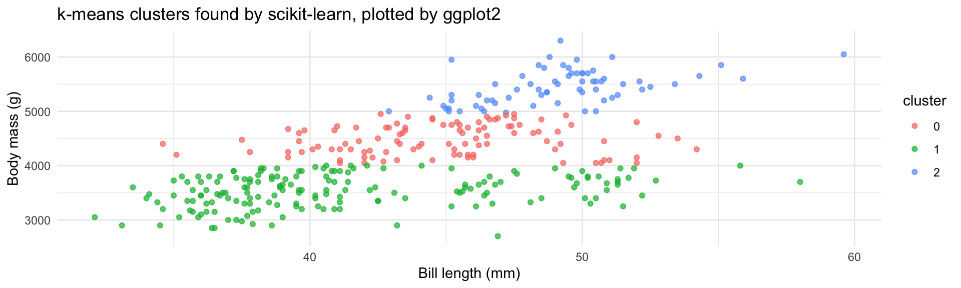
A round trip: R data → Python model → R plot

The good-practice pattern: R wrangles, Python models, R visualises.

from sklearn.cluster import KMeans

X = r.penguins[["bill_length_mm", "body_mass_g"]].dropna()
clusters = KMeans(n_clusters=3, n_init=10, random_state=13).fit_predict(X)

py$X |>
  mutate(cluster = factor(py$clusters)) |>
  ggplot(aes(bill_length_mm, body_mass_g, colour = cluster)) +
  geom_point(alpha = 0.7) +
  labs(x = "Bill length (mm)", y = "Body mass (g)",
       title = "k-means clusters found by scikit-learn, plotted by ggplot2") +
  theme_minimal()

• Full circle in ~10 lines: r.penguins into Python, sklearn clusters, py$ back into a dplyr/ggplot pipeline
• Compare clusters to the true species from earlier scatter — they roughly recover Gentoo vs the rest on these 2 features
• This is the slide to remember for projects: each language does what it’s best at, no CSV files in between

Importing Python modules directly in R

No Python chunks needed — import() gives you the module as an R object:

np <- import("numpy")

np$median(c(1, 3, 5, 100))

[1] 4

np$linspace(0, 1, num = 5L)

[1] 0.00 0.25 0.50 0.75 1.00

Important

Note the 5L: many Python functions insist on integers, but R numbers are doubles by default — num = 5 would error. The L suffix is the most common reticulate stumbling block.

• $ walks the module: np$linspace == numpy.linspace; autocomplete works in RStudio
• Demo the failure live if time: np$linspace(0, 1, num = 5) → “expected integer”
• This style suits “I need ONE function from a Python library” — chunks suit larger Python blocks

When to use which language?

Reach for R

• data wrangling & cleaning (dplyr, tidyr)
• statistical inference & modelling
• visualisation (ggplot2) & tables (gt)
• reports, websites, dashboards (Quarto, Shiny)

Reach for Python

• machine learning (scikit-learn)
• deep learning & LLMs (PyTorch, transformers)
• when the best library for the job is Python-only
• gluing services, APIs, and pipelines together

Tip

Good practice: pick one primary language per project and borrow from the other via reticulate where it clearly wins. Document the Python dependency (e.g. a requirements.txt) just like you document R packages with renv.

• The worst setup is a 50/50 split where every reader needs to master both — borrow, don’t blend
• Reproducibility angle ties back to week 9: a reticulate project has TWO environments to pin
• For their course projects, R remains the primary language — Python is an option, not an expectation

Try it live

Tomorrow’s practical, in one slide — given this Python file stats_helpers.py:

def total(numbers):
    """Return the sum of a list of numbers."""
    result = 0
    for n in numbers:
        result += n
    return result

Use it from R:

daily_steps <- c(8500, 12000, 9300, 400)
py$total(daily_steps)

[1] 30200

• If time permits: open practical.qmd and run Ex 1.2 live instead of this slide
• Ask before running: what does result += n do? (compound assignment, result <- result + n)
• Then ask: is this loop good Python? (No — sum(numbers) or numpy; the practical discusses this)

BONUS: Installing Python

Want Python on your own machine? Ways to get it, in order of recommendation:

1. uv — fast, modern manager for Python versions, environments, and packages

   uv venv .venv && uv pip install pandas seaborn

2. Anaconda / Miniconda — classic data science distribution; heavier, but everything included

3. python.org installer — not recommended: no environment management, easy to end up with conflicting global packages

Tip

No install needed to experiment: reticulate::py_require("pandas") can provision a Python environment for you automatically (reticulate ≥ 1.41 downloads its own via uv). Details in the practical.

• Virtual environments per project == renv for Python; same reproducibility logic as week 9
• python.org installs aren’t broken, but beginners end up with PATH chaos and global package soup
• The py_require route is the lowest-friction path for the practical — no admin rights needed

BONUS: The other direction — R from Python

rpy2 embeds R inside Python — reticulate’s mirror image:

import rpy2.robjects as robjects

rsum = robjects.r["sum"]        # grab R's sum()
rsum(robjects.FloatVector([1.5, 2.5, 3.0]))   # returns 7.0

robjects.r("t.test(rnorm(100), mu = 0)")      # any R code as a string

• Useful when a team’s main stack is Python but one step needs an R package (e.g. a specific statistical test or mixed-model routine)
• Rougher edges than reticulate — conversions are more manual
• In Quarto you rarely need it: mixed R + Python chunks (like this deck) usually solve it more cleanly

• Not today: Let’s go to RStudio!
• Static example (not executed) — rpy2 isn’t installed here, and that’s fine for a pointer slide
• Mention: pandas even had rpy2-based R interop built in historically; the pattern is common in industry
• Take-away: interop is a two-way street; the skill is knowing it exists, not memorising APIs

Summary

Limitations of R

• R is a domain-specific language — unbeatable for statistics and visualisation, weaker as a general-purpose tool
• Copy-on-modify semantics and interpreted loops can cost memory and speed — vectorise, or reach for another language
• OOP is fragmented (S3, S4, R6, S7) where most languages have one class system
• Some ecosystems (deep learning, production ML, web backends) live primarily in Python

Python fundamentals

• Python is a general-purpose language; data science lives in libraries: pandas, numpy, matplotlib/seaborn, scikit-learn
• Core containers: lists [ ], dictionaries {k: v}, tuples ( ), sets { } — and indexing starts at 0
• Methods are called on objects (df.groupby(...).mean()) instead of functions on data (aggregate(...))
• dplyr verbs and ggplot2 layers have direct pandas / seaborn counterparts — the concepts transfer, only the syntax changes

{reticulate}

• Runs an embedded Python session inside R — one shared workflow, two languages
• Objects convert automatically: vector ↔︎ list/array, data.frame ↔︎ pandas DataFrame
• Access Python from R via py$x, R from Python via r.x; load functions with source_python() or import()
• Use each language where it is strongest: e.g. R for wrangling, visualisation and inference; Python for ML and specialised libraries

This week’s practical & reflection

• Practical tomorrow: read & translate Python snippets, then call a Python function from R with reticulate — plus project time for the final submission (22 Jul)
• Reflection log: what surprised you when switching between R and Python? Did an LLM help bridge the gap — and did you verify its output?

Upcoming deadlines

Final submission 22 Jul · Individual contribution statement 23 Jul · Oral exam 29 Jul

Resources

• reticulate documentation — Python in R: setup, object conversion, source_python() and import()
• Python for R Users — a full “R to Python” guide, written for people who already think in R

• Both links are in tomorrow’s practical too — point students there for self-study
• Python for R Users is the single best follow-up if anyone wants to go deeper