Advanced Statistical Programming using R
Week 14: Course Review & Oral Exam Prep
2026-07-16
Announcements
- Final submission due 22 Jul (group repo)
- Individual contribution statement due 23 Jul (Moodle).
- Oral exam 29 Jul.
- Oral exam times and zoom links will be sent out tomorrow (Fri Jul 17)
This Week
- Part 1: Course review
- Part 2: Oral exam — format, topics, how to prepare
Course Review
- Course objectives
- W1-11 Review
Course philosophy
- Developing data analysis ‘why’, ‘what’ & ‘how’ > learning a limited set of R skills
- Deliberate and strategic usage of AI assistance in data science
- Part 1: Foundations & developing ‘taste’
- Part 2: Application & practising ‘implementation’
- Incremental artefacts:
- Solo reflection log
- Collaborative project
- Oral exam
Syllabus
Part 1: Statistical Programming Foundations
- W02: Scripts, Functions & Refactoring
- W03: Debugging
- W04: Version Control & Remotes
- W05: Quarto Websites & Collaborative Coding
- W06: R Packages
Part 2: Working with Real World Data
- W07: Initial Data Analysis & Data Cleaning
- W09: Reproducibility, Open Data & renv
- W10: Analysis & Inference
- W11: Statistical Communication & Visualisation
Part 3: Advanced Topics & Summary (Not Examined!)
- W12: Interactive Data Storytelling
- W13: Multi-lingual Analysis (Python/R)
- W14: Review & Outro
Statistics + Programming = Learning from Data
This course aims to support you in learning from data using statistical reasoning AND computational tools.
Statistical
- thinking,
- inference,
- visualisation,
- modelling,
- and communication
Programming
- R packages and workflows
- code style and quality
- reproducibility practices
- version control & collaboration
- LLMs & generative AI
Data Science Workflow
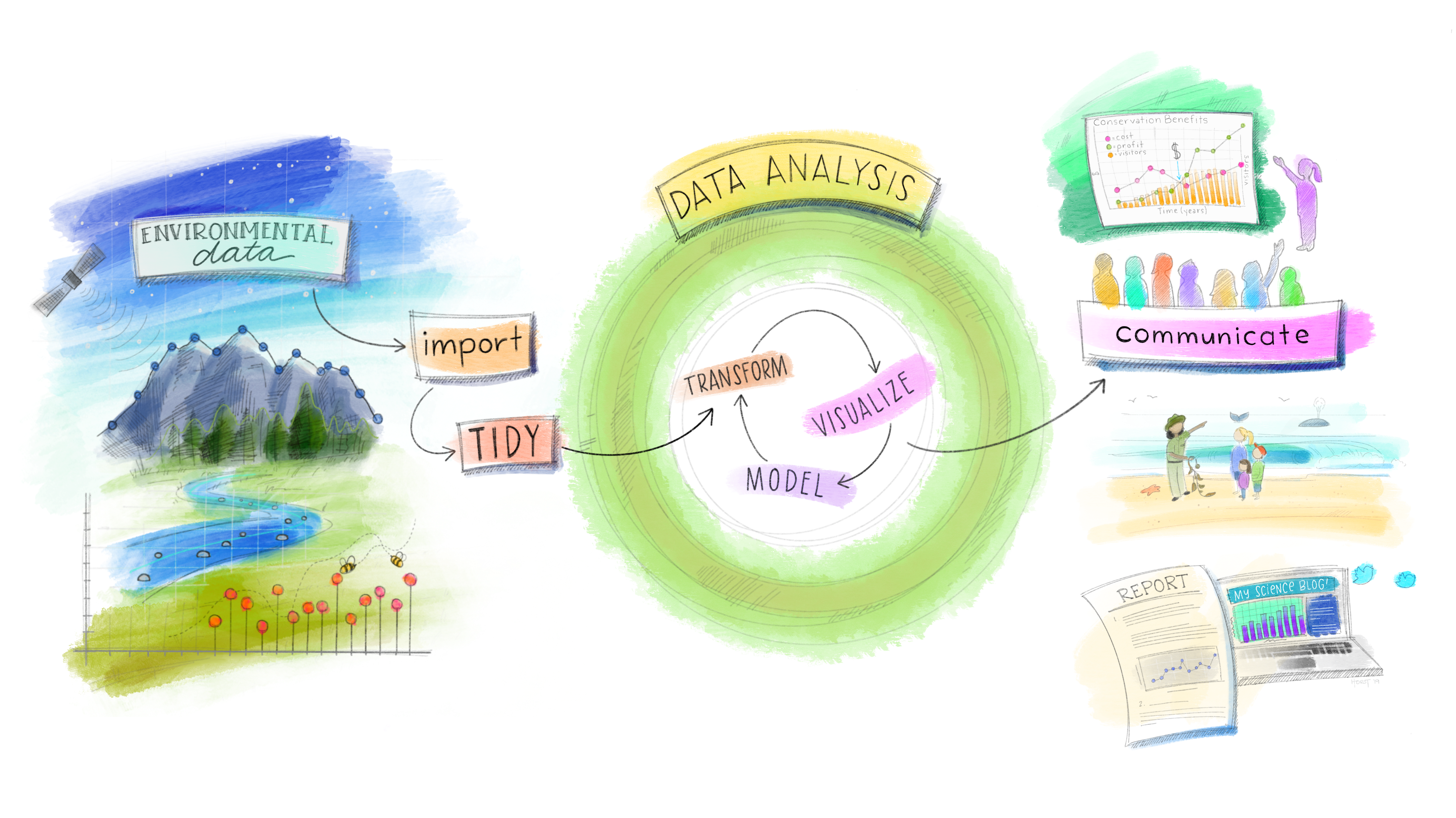
Part 1: Statistical Programming Foundations
W1: Command Line Interface
- What is the command line?
- What can you do from the command line?
- create, delete and navigate folders and files
- run and install programs
- What is the “working directory”? How do you find out your current working directory?
Command Line
Navigate
Create & remove
Tip
Windows uses cd for pwd, dir for ls, type for cat, and del for rm.
W2: Functions in R
- How to write valid functions
- How to test functions
- How to break down data analysis workflows into smaller tasks (or functions)
- Style considerations for function names, error messages and interfaces
- How to design Don’t Re-Read Yourself functions
Function Syntax in R
| Part | What it does |
|---|---|
function(arg1, arg2 = default) |
declares the function and its inputs |
{ ... } |
body — the code that runs |
return(...) |
what the function hands back (optional) |
Tip
If there is no return(), R returns the value of the last expression.
Testing & Validating Functions
Test on known inputs, then stress-test
Warning
R coerces types silently — wrong answers with no error are worse than a crash.
Validate inputs explicitly
stopifnot() — quick but blunt:
if / stop() — custom message:
“you gave me THIS, but I need THAT”
Strategies for better functions
DRY → DRRY
- DRY: Don’t Repeat Yourself
- copy-paste 3 times → write a function (targets repetition)
- DRRY: Don’t Re-Read Yourself
- re-read a block 3 times → improve a function (targets cognitive load)
Outside-In vs Inside-Out
- Outside-In: write the call before the body — design the interface first
- Inside-Out: start with working code, chunk it into named ideas, then abstract
Tip
If you struggle to name a function, it’s probably doing too many things.
Don’t Re-Read Yourself Functions
Outside in:
Name: What am I trying to do? What evokes the action
Inputs: What pieces of information do I need to provide?
Output: What are we returning?
Inside out:
Copy text into body
Identify complexity to manage
Abstract the complexity
W3: Debugging in R
- What types of conditions are there in R?
- What kinds of steps or strategies can you use for troubleshooting?
- Where can you get help?
- What should you consider when using LLMs for help?
- What should you include when asking for help in R?
- What is a minimal reproducible example, and what should be included?
- What are trackbacks?
R Help
- Read the message — it tells you where (function) and why (what went wrong)
- Troubleshoot first: search the message, divide & conquer, restart R, read the docs
- Ask well: write a minimal reproducible example (MRE); use
{reprex}to format it - Where to ask: Moodle forum, Stack Overflow (
[r]), Posit Community
Errors & Troubleshooting
Three condition types
| Type | What to do | |
|---|---|---|
| 🚨 | Error | Must fix |
| ⚠️ | Warning | Inspect output |
| 💬 | Message | Read it |
Troubleshooting steps
- Read the message
- Search the message
- Divide and conquer
- Read the docs
- Restart R
Minimal Reproducible Examples
Minimal
- Remove unrelated code
- Limit package dependencies
- Use built-in datasets or synthetic data
Reproducible
- Include
library()calls - Use
dput()for real data - Set
set.seed()if randomness is involved
Tip
Writing a reprex often finds the bug for you — making code self-contained reveals missing library() calls or stale variables.
Debugging Tools
| Goal | Tool |
|---|---|
| Locate where the error occurred | traceback(), rlang::last_trace() |
| Pause and inspect inside your function | browser() |
| Debug a package function without editing it | debugonce(fn), debug(fn) |
| Debug outside R (YAML, paths, render) | quarto render in terminal |
W1: Basics of Version Control
- What are version control systems (VCS)?
- What are the benefits of using VCS?
- What is git repository?
- What is the git commit workflow?
Basic Git Commands
Set up & inspect
Stage & commit
The three areas
working directory  →  staging area  →  repository
   (your files)       (git add)        (git commit)
Think of it as:
- Edit files as normal
- Stage the changes you want to keep (
git add) - Commit a named snapshot (
git commit)
W4: GitHub & Collaborative Coding
- What makes for a good git message?
- How to view the history of a git repository?
- How to restore removed files?
- What files should not be tracked in git?
- How to prevent tracking of certain files?
- What is a remote repository?
- What is the difference between forking and cloning repositories?
- What is the workflow for working with remotes?
Git: local version control
init,add,commit— the core loop; each commit is a snapshot with a parent pointer- Good commit messages are imperative, one logical change at a time
- Use RStudio’s History panel (or
git log) to browse and restore past versions - Specify files you don’t want to track with
.gitignore
GitHub: beyond local
If you already have a local repo
-u sets origin/main as the upstream — after this, plain git push works.
Tip
git remote -v confirms the connection — you should see origin pointing to your GitHub URL.
Pull before you push!
git pull— fetch and merge any remote changes first- Resolve any conflicts if they arise
git push— send your commits to GitHub
Tip
Make it a habit: pull first, then push. This avoids most “rejected push” errors.
W5: Collaborative Coding
- What are git branches? When should you use each?
- What is a merge?
- What kind of merge conflicts can you encounter?
- How to resolve merge conflicts?
Collaborative Coding with Git
Branches, stash & worktrees
- Work on features in isolation —
git switch -c <name> - Stash unfinished work to switch context —
git stash/git stash pop - Use
git worktreewhen you need two branches open at once
Pull requests & conflicts
- Push your branch with
git push -u origin <name>, then open a PR on GitHub - Collaborators review, comment, and approve before merging
- Resolve conflicts by editing the
<<<<<<<markers,git add, thengit commit
Tip
Pull at the start of every session, push at the end — this keeps conflicts small.
W5: Quarto Websites
- What are the components of a Quarto Document?
- How to render a Quarto document
- What’s the difference between a webpage and website?
- How to publish a Quarto website
Quarto Websites
- A Quarto project is a folder with
_quarto.yml— it renders all.qmdfiles and shares options across them - A Quarto website adds shared navigation, search, and a footer; deploy to GitHub Pages with
quarto publish gh-pages - Share code display options (
code-fold,code-line-numbers) underformat: html:and execution options (echo,freeze) underexecute:in_quarto.yml
Quarto & Project Structure
- A reproducible project keeps raw data read-only, separates code from outputs, and documents everything in
.qmdfiles _quarto.ymlrenders the whole repo as a website — proposal, report, and README in one place- Render early, render often — catch broken code before submission
W6: R Packages
- What is an R Package?
- How are R Packages structured?
- What are the benefits of R packages?
- What is the R Package development workflow?
- How to add data into an R Package
- What types of documentation are available for R Packages?
- Stylistic considerations for good R packages
R Packages
- A package is the standard unit for sharing functions, data, and documentation in R
usethis&devtoolshelp to streamline package development- Data packages (e.g.
munichvisitors) distribute clean, documented datasets — a great first package roxygen2turns#'comments into.Rdhelp files — document as you write
Development workflow
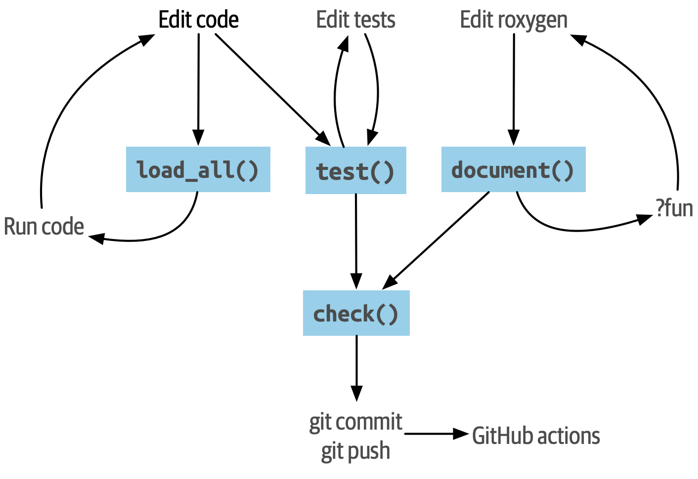
Documentation & Design
- Every exported object needs
@param,@returns,@export, and@examples - Expose data as an argument (
data = museum_visitors) when users may want to filter or swap it - Package scope:
- Coherent theme — Group functions with shared theme
- Limit dependencies — every imported package is a liability your users inherit
- Package design:
- Single responsibility — Functions should be limited to one function or idea
- Consistent interfaces —
datafirst, options last with sensible defaults
Tip
Ask: if a colleague installed this tomorrow with no context, would the function names tell them what to call and when?
Part 2: Working with Real World Data
W7: IDA, screening, cleaning, missingness
- What are the goals of IDA, EDA and CDA?
- What tasks fall under IDA?
- What issues can be detected in IDA?
- What is data screening? data quality? data cleaning?
- What needs to be considered when you have missing data?
IDA: Key ideas
- IDA is a systematic pre-analysis step — it checks data integrity without touching the research questions
- IDA issues occur at univariate, multivariate, and dataset levels — check all three
- Tidying (reshape/rename) ≠ cleaning (fix values/types) ≠ screening (characterise) — they overlap but have different goals
- All preparation decisions must be documented and justified in a reproducible script
Screening: Data types & formats
- Declare column types explicitly on import — avoid relying on guessing
- Use
lubridatefor dates; other specialist packages for geospatial (sf), time-of-day (hms), factors (forcats) etc. - Check every column: does the R type match the real-world meaning of the variable?
- Use
glimpse()for the whole table;str()for a single column
Cleaning: tools & fixes
- Plot first — histograms, boxplots, and line plots reveal issues that
summary()hides - Hypothesise before fixing — ask why a value looks wrong before deciding how to handle it
- Variable-level: recode types (
as.*()), flag/replace out-of-range values, standardise encodings - Structural: remove duplicates (
distinct()), reshape (pivot_*()), split/merge columns (separate(),unite()) - Not handling missingness is itself a decision — document it either way
Missingness
- Explicit missingness (
NA) — visible; find withis.na(),summary(),naniar::vis_miss() - Implicit missingness — absent rows; requires domain knowledge about expected structure
- Use
tidyr::complete()ortsibble::fill_gaps()to make implicit missingness explicit - The missing data mechanism (MCAR / MAR / MNAR) determines whether dropping or imputing is valid
W9: Reproducibility, Open Data & renv
- Why is reproducibility important?
- What are the different types of reproducibility?
- What is renv?
- How to use renv in an R project?
- What is open data? What are different types of openness?
W9: Documenting data science
- What might we document in a data science workflow?
- What should be included when documenting datasets?
- How does documentation vary across IDA, EDA, CDA?
Reproducibility
- Computational reproducibility: same data + same code → same results
- renv fixes package versions; Docker fixes the full environment; Quarto + Git handle code and narrative
- Reproducibility is a means — the goal is trustworthy, reusable, cumulative knowledge
renv
renv::init()creates a project-local library and records versions inrenv.lockrenv::snapshot()updates the lockfile;renv::restore()rebuilds the library from it- Commit
renv.lockto git; addrenv/library/to.gitignore
Open Data
- Legal openness: know how to read and apply licences (CC0, CC BY, ODbL)
- Technical openness: use standard, open formats (CSV, plain text)
- FAIR: data should be Findable, Accessible, Interoperable, Reusable
- Always document the licence, provenance, and context of any dataset you use
Documenting data analyses
- Document decisions, not just actions — why at every stage (IDA, EDA, CDA)
- Keep a reproducible script from raw data to clean data in
data-raw/ - State hypotheses before testing; disclose any deviations from plan
- Well-organised data: consistent names,
YYYY-MM-DDdates, one value per cell, plain text files
W10: Analysis & Inference
- What role does inference play in different types of analysis?
- What issues can arise with multiple testing?
- How to specify and implement hypothesis tests
Learning from data
- Three goals:
- descriptive (what is the state of things?),
- explanatory (is there a real relationship?),
- predictive (does this generalise?)
- Exploratory vs confirmatory is orthogonal to the goal — any analysis type can be either; the distinction is whether the question was fixed before looking
- Inference tools differ by goal: CIs for descriptive, hypothesis tests + effect sizes for explanatory, held-out evaluation for predictive
Planning for inference
- A data analysis plan covers the full project; an inference plan is the component where you generalise beyond your sample
- Running tests after exploring is normal — label those findings as exploratory/candidate and treat them as hypotheses for future work
- Each look at the data spends some of the evidentiary budget — standard tools don’t adjust for this automatically
- Write it down: even a paragraph before you start is enough to separate what you planned from what you discovered
{infer}
- Workflow:
specify()→assume()→calculate()→visualize()/get_p_value() assume("t" / "z" / "Chisq" / "F")uses the same theoretical distributions as Stat 1/2- The null plot shows you where your test statistic sits in the null distribution
- Extension:
generate()simulates the null without assuming a distribution
W11: Statistical Communication & Visualisation
- What kinds of statistical information need communicating?
- How to choose between tables and plots?
- How to format tables
- How to improve the clarity and effectiveness of plots
Communicating with Tables
- Choose between tables and plots based on your message and audience – which matter more? pattern or trend or exact values?
- Descriptive summaries can cover: variable list, observation count, missing values, distributions, and correlations
- Model result tables show estimates, uncertainty (SE or CI), and a fit statistics — use
broom::tidy()to get a tidy data frame first - Correlation tables and plots:
{corrr}produces tidy correlation data frames ready to pipe intogt()orrplot() - Cross-tabulations show joint frequency distributions —
count()+pivot_wider()+gt()is the standard pipeline - Combine tables and visualisations when you need both precision and pattern:
formattablecolour tiles are one lightweight option
Making tables with {gt}
- The
gtworkflow: wrangle first, thengt(), then stack formatting (fmt_*), column (cols_*), and annotation (tab_*) layers - Column labels should carry units (
mm,g,%) — keep cells clean withcols_label()andhtml()/md()helpers tab_spanner()groups related columns under a shared header- Right-align numbers, left-align text; choose decimal places to match the precision that matters to your reader
- Every table should have a title and a source note;
- Captions should state the take-away, not just repeat the title
- Alt text for tables is set via
tbl-capin Quarto — write what a screen reader needs to understand the finding
Communicating with Visualisation
- Start with intent!
- what relationship do you want to show?
- who is the audience?
- Iterative improvement
- start with a default chart, then adjust encodings, labels, and scale to foreground the message
- does your chart match your message?
- consider perceptual tasks and hierarchy as a guide
- Supporting text
- The subtitle should state the finding, not just repeat the axes; the caption credits the data source
- Alt text (
fig-altchunk option) conveys the chart’s message — not its structure — for screen readers
Advanced Topics
Interactive visualisation
- htmlwidgets (
plotly,leaflet,DT) add interactivity to any Quarto HTML output — no server required ggplotly()is the quickest path from aggplot2plot to an interactive one- Observable JS in Quarto enables reactive, filter-driven views without a Shiny server
- Shiny is the right tool when you need server-side computation or persistent state
Geospatial visualisation
{sf}+geom_sf()for choropleth and boundary maps with proper projection handling{geofacet}for small-multiple comparisons arranged in a geographic layout- Choose based on whether exact geography or spatial comparison of trends is the goal
Limitations of R
- R is a domain-specific language — unbeatable for statistics and visualisation, weaker as a general-purpose tool
- Copy-on-modify semantics and interpreted loops can cost memory and speed — vectorise, or reach for another language
- OOP is fragmented (S3, S4, R6, S7) where most languages have one class system
- Some ecosystems (deep learning, production ML, web backends) live primarily in Python
Python fundamentals
- Python is a general-purpose language; data science lives in libraries:
pandas,numpy,matplotlib/seaborn,scikit-learn - Core containers: lists
[ ], dictionaries{k: v}, tuples( ), sets{ }— and indexing starts at 0 - Methods are called on objects (
df.groupby(...).mean()) instead of functions on data (aggregate(...)) dplyrverbs andggplot2layers have directpandas/seaborncounterparts — the concepts transfer, only the syntax changes
{reticulate}
- Runs an embedded Python session inside R — one shared workflow, two languages
- Objects convert automatically: vector ↔︎ list/array, data.frame ↔︎ pandas DataFrame
- Access Python from R via
py$x, R from Python viar.x; load functions withsource_python()orimport() - Use each language where it is strongest: e.g. R for wrangling, visualisation and inference; Python for ML and specialised libraries
Oral Exam
Format
- 15 min per student
- Individual, online, 29 Jul
- 5 Topics. At least one question per topic.
- With a group project – starting questions will be personalised to your repo (primarily based on
group-reflection.qmd)
Topics
| Topic | Potential Sub-topics |
|---|---|
| R programming | functions · debugging · R packages |
| General programming & workflow | git · CLI · renv · Quarto websites |
| Data preparation & analysis | IDA (glimpse) · hypothesis testing (infer) · open data principles |
| Statistical communication | tables (gt) · plots (ggplot2) · documenting data analyses |
| Project management | project organisation · collaborative practices · LLM usage |
What’s assessed
- Questions will include:
- project/application questions,
- course content (from W1–W11),
- and synthesis across topics
- For group work — make sure you can speak to both your contributions and what your group achieved together
- Demonstrate engagement with the course and statistical programming with real world data
How to prepare
- Review lecture and practical material for each sub-topic — the exam draws directly on both, not just slides
- If you did the project: be ready to discuss decisions and reflections,
- If you didn’t: practice reasoning from scratch on datasets from the lectures or practical
- Expect cross-topic questions (e.g. git merges → collaborative practices) — think about how weeks connect, not just within one week
Sample Questions: R Packages
munichvisitors/
├── DESCRIPTION
├── R/
│   └── plot_museums.R
├── data/
│   └── museum_visitors.rda
├── data-raw/
│   └── museum-visitors.R
└── README.Rmd
Course Content
- What’s the difference in purpose between
data-raw/anddata/? - Why does that split matter for reproducibility?
Sample Questions: Project Organisation
.
├── CONTRIBUTING.md
├── README.md
├── _quarto.yml
├── code
│   ├── 01_download.R
│   ├── 02_clean.R
│   ├── 03_eda.R
│   └── 04_analysis.R
├── data
│   ├── processed
│   └── raw
│       └── LICENCE.txt
├── docs
├── index.qmd
├── our-statprog2-project.Rproj
└── proposal.qmd
Reflection
- How did your project repo structure evolve over the semester — what changed, and why?
- If you started the project again, what would you structure differently from day one?
Cross-topic synthesis:
- (→ collaborative practices) Did your repo structure change at all once more than one person started committing to it?
- (→ CLI) If a new group member cloned your repo, what terminal commands would they need to run to get oriented?